Logistic Regression in R: From glm() to Odds Ratios, ROC, and AUC
Logistic regression predicts the probability of a binary outcome by passing a linear combination of predictors through the sigmoid function. In R you fit it in one line with glm(family = binomial), read the coefficients on the log-odds scale, exponentiate them to get odds ratios, and evaluate the classifier with confusion matrices, ROC curves, AUC, and a calibration check.
How do you fit a logistic regression in R?
The function for logistic regression in R is glm() with family = binomial. Hand it a 0/1 outcome, one or more predictors, and a data frame, and it returns a fitted object with coefficients, standard errors, z-values, and p-values, all on the log-odds scale. The example below uses the built-in mtcars data and predicts whether each car has a manual transmission (am = 1) or automatic (am = 0) from weight (wt) and horsepower (hp).
The summary() printout is the most important single object in this whole tutorial. Every interpretation later in the post comes back to numbers you can already see in it.
Read the coefficient column first. wt is negative, so heavier cars are less likely to be manual once you control for horsepower. hp is positive, so among cars of similar weight the more powerful ones lean manual. Both p-values sit under 0.05, which means each predictor adds signal beyond chance. The deviance dropped from 43.2 (intercept-only model) to 10.1 (the fitted model), a sharp reduction that tells you the predictors are doing real work. Hold on to this object as fit_simple, every later block reuses it.
family = binomial is the idiomatic form. Both family = binomial and family = "binomial" work, but the unquoted version is what you will see in R documentation, textbooks, and most production code. Stick with it for consistency.Try it: Fit a one-predictor model ex_fit of am on wt alone and check whether the weight coefficient is still negative and significant.
Click to reveal solution
Explanation: Weight alone still pushes strongly in the negative direction. Notice the coefficient (-4.02) is smaller in magnitude than in the two-predictor model (-8.08); when hp is removed, wt no longer needs to overshoot to compensate for the positive hp term.
Why does linear regression fail for binary outcomes?
The temptation is real: an outcome is just a number, so why not throw it into lm() and read off the slope. The answer is that lm() will produce numbers, but they will not behave like probabilities. You can see that with a single line of code: ask the linear model to predict three made-up cars, and at least one prediction will fall outside [0, 1].
The first prediction says 118% probability of manual transmission, and the third says -53%. Neither is meaningful. That is the surface problem. The deeper problem is that the residuals from a linear fit to a 0/1 outcome cannot be normally distributed (the truth is always 0 or 1, so residuals always pile up at two values), which invalidates every standard error and p-value lm() would print. Logistic regression solves both issues at once: keep the linear combination of predictors, but pass it through a function that maps any real number into [0, 1]. That function is the sigmoid.
The curve flattens to 0 on the left, to 1 on the right, and crosses 0.5 exactly when the linear predictor equals 0. That is the geometric heart of logistic regression: a plain weighted sum of predictors, squashed through this S-shape, becomes a probability.
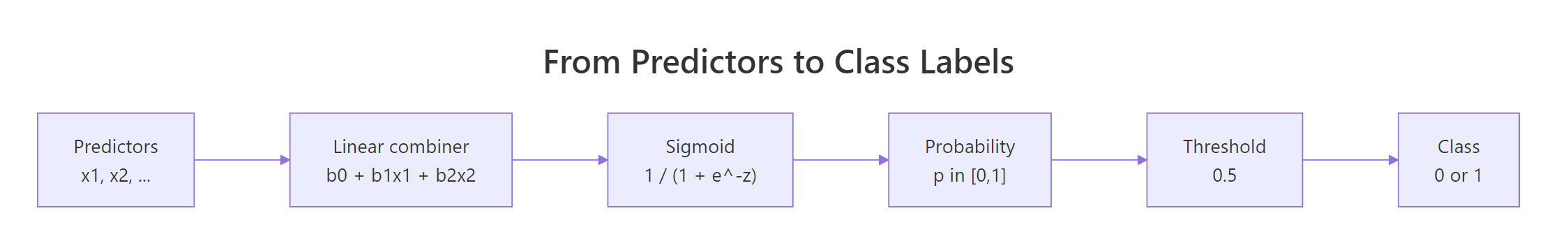
Figure 1: How logistic regression turns predictor values into a class label.
The model can also be written in one equation: the log-odds of the outcome are linear in the predictors.
$$\log\left(\frac{p}{1 - p}\right) = \beta_0 + \beta_1 x_1 + \beta_2 x_2 + \dots$$
Where:
- $p$ = probability the outcome equals 1
- $\frac{p}{1-p}$ = the odds (a positive number; not bounded above)
- $\log\bigl(\tfrac{p}{1-p}\bigr)$ = the log-odds, also called the logit (any real number)
- $\beta_0, \beta_1, \dots$ = the coefficients R estimates
Solve for $p$ and you get back the sigmoid: $p = 1 / (1 + e^{-z})$ with $z = \beta_0 + \beta_1 x_1 + \dots$. The two formulations are equivalent.
Try it: Write a function ex_sigmoid(z) that returns 1 / (1 + exp(-z)), then test it on 0 and 2 to verify the curve.
Click to reveal solution
Explanation: At z = 0 the sigmoid hits 0.5 exactly, the decision boundary. By z = 2 the probability has already climbed to about 0.88, so a moderately positive linear predictor produces a high probability of the positive class.
How do you interpret coefficients as odds ratios?
Coefficients on the log-odds scale are awkward to talk about. Exponentiating them produces odds ratios, which are easier: a multiplier on the odds of the positive outcome per one-unit increase in the predictor. An OR of 1 means no effect, OR > 1 means the odds go up, OR < 1 means the odds go down.
The relationships between probability, odds, and log-odds are worth burning into memory because every logistic regression table sits on top of them.
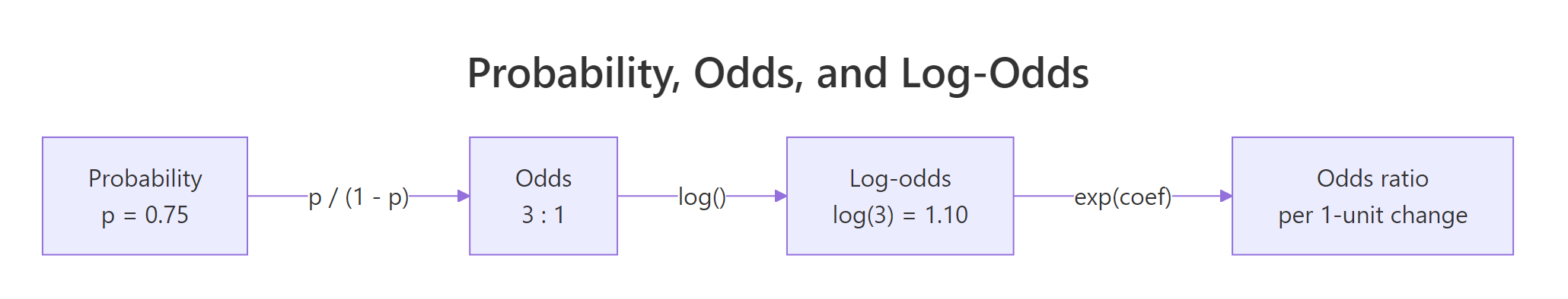
Figure 2: Probability, odds, and log-odds are three views of the same quantity.
The cleanest way to produce odds ratios with confidence intervals is broom::tidy() with exponentiate = TRUE and conf.int = TRUE. One call returns a tibble with estimates, CIs, and p-values, ready for a report.
Read the estimate column as odds ratios. For wt, each extra 1000 lbs multiplies the odds of a manual transmission by about 0.0003, an enormous decrease. For hp, each extra horsepower multiplies the odds by about 1.04, a 4% per-hp increase. The 95% CI for hp runs from 1.00 to 1.08, so the direction is solid but the magnitude is uncertain. The intercept's odds ratio of 156 million is the odds at wt = 0 and hp = 0, a weightless car with no engine, which is why intercept ORs are usually ignored.
broom::tidy(fit, exponentiate = TRUE, conf.int = TRUE) is the one-liner you want. It is easier to read and report than stitching exp(coef(fit)), exp(confint(fit)), and summary(fit)$coefficients together by hand. The result drops straight into knitr::kable() or gt::gt() for publication-ready tables.p = 0.5 doubling the odds is a noticeable jump, but near p = 0.01 or p = 0.99 the probability barely budges. Translate ORs back to probabilities at the values you actually care about before claiming a real-world effect size.Try it: Pull the odds ratio for hp out of or_table and store it in ex_or_hp, then read what it means in plain English.
Click to reveal solution
Explanation: Each additional horsepower multiplies the odds of a manual transmission by about 1.04, holding weight constant. Compounded over 100 hp, that becomes 1.04^100 ≈ 38, which is why the predicted probability climbs so steeply with horsepower in this dataset.
How do you predict probabilities and build a confusion matrix?
predict() on a glm defaults to the link scale (log-odds), which is rarely what you want. Pass type = "response" to get probabilities. Then apply a threshold (0.5 is the textbook default) to turn probabilities into 0/1 predictions, and tabulate against the actual outcomes.
Every row of mtcars now has a predicted probability of being manual, ranging from near 0 to near 1. The Mazda RX4 (probability 0.88) is correctly identified as a likely manual; the Hornet 4 Drive (0.16) as automatic. Now apply the 0.5 cutoff and build the confusion matrix.
The classifier got 30 of 32 cars right, which is 93.75% accuracy. The matrix shows one false positive (an automatic predicted as manual) and one false negative. On 32 rows that is impressive but slightly suspect: the model was scored on the same data it was fit on, which always flatters the result. A real evaluation would split into train and test, or use cross-validation.
Try it: Recompute the confusion matrix at threshold 0.3 instead of 0.5, then save the new accuracy to ex_acc.
Click to reveal solution
Explanation: A lower threshold catches more positives but classifies more negatives as positives, so accuracy drops. Whether that is a worthwhile trade depends on which kind of mistake costs more.
How do you evaluate the model with ROC curves and AUC?
A confusion matrix freezes one threshold. The ROC curve (Receiver Operating Characteristic) sweeps every possible threshold and plots the true-positive rate (sensitivity) against the false-positive rate (1 − specificity). The area under that curve, the AUC, summarises the entire tradeoff in a single number: 0.5 is random guessing, 1.0 is perfect separation, and 0.8 or above is generally considered strong.
The pROC package is the standard tool. Pass it the truth vector and the predicted probabilities, and it returns an roc object that you can plot or pass to auc() and ci.auc().
The curve hugs the top-left corner, the visual signature of a strong classifier. The AUC of 0.98 has a clean interpretation: pick one manual and one automatic car at random, and the model assigns a higher predicted probability to the manual one about 98% of the time. That is excellent ranking quality, with the same caveat as before: it was measured on training data.
A point estimate of AUC without a confidence interval can be misleading. ci.auc() returns a 95% CI by DeLong's method.
The interval runs from 0.94 up to the theoretical ceiling of 1.0. With only 32 rows the CI is wide; in practice you would want more data before claiming this AUC as a property of the population, not just this sample.
pROC::coords(roc_obj, "best") returns the Youden-optimal threshold. Youden's J statistic is sensitivity + specificity − 1, and coords maximises it by default. Using it is a defensible automatic choice when false positives and false negatives carry equal cost.Try it: Use coords(roc_obj, "best") to extract the Youden-optimal threshold, store it in ex_best, and compare it to the default 0.5.
Click to reveal solution
Explanation: The Youden-optimal cutoff is about 0.39, well below the textbook 0.5. At that threshold the model catches every actual manual (sensitivity = 1.0) while misclassifying only one automatic (specificity ≈ 0.95). On this dataset that beats the default cutoff on both axes.
How do you check model fit and calibration?
A high AUC proves the model ranks cases correctly: positives get higher probabilities than negatives on average. It says nothing about whether the predicted probabilities are honest. A classifier that always predicts 0.9 for positives and 0.8 for negatives can have AUC = 1 yet still be badly miscalibrated. If a downstream system is going to plug these probabilities into a formula (risk score, expected loss, regulatory report), calibration matters as much as ranking.
The first calibration check costs nothing extra. McFadden's pseudo-R² is one minus the ratio of model deviance to null deviance, both of which glm already computed. Values above 0.2 are considered good for logistic regression; the scale is not the same as ordinary R² and 0.5 is unusually high.
A pseudo-R² of 0.77 is very high, again reflecting how tightly this 32-row dataset fits. Real-world logistic models more typically land between 0.1 and 0.4.
For calibration, a binned table is more revealing than any single statistic. Divide the predicted probabilities into a few bins (here, quintiles), then compare the mean predicted probability and the mean observed outcome inside each bin. If the model is calibrated, the two columns should track each other.
The two rightmost columns sit close to each other in every bin, the pattern you want to see. Bin 3's predicted mean of 0.27 lines up with an observed rate of 0.29; bin 4's 0.72 matches 0.83. The probabilities behave like probabilities here, which means downstream code can treat them as risks rather than just rankings.
Try it: Recompute the pseudo-R² directly from fit_simple's deviance slots without the intermediate variables, and store the result in ex_pr2.
Click to reveal solution
Explanation: Both deviance values live directly on the fitted glm object, so there is no need to rerun summary(). McFadden's formula is the one-liner above and runs in microseconds.
Practice Exercises
Exercise 1: Odds-ratio table for a different model
Fit a logistic regression of am on mpg + qsec in mtcars and return a tibble of odds ratios with 95% confidence intervals using broom::tidy. Save the result to my_or_table.
Click to reveal solution
Explanation: The OR for mpg is about 2.7, so each extra mile per gallon nearly triples the odds of a manual transmission, fuel-efficient cars in this dataset tend to be manuals. qsec (quarter-mile time) has an OR of 0.19, so slower cars are less likely to be manuals.
Exercise 2: End-to-end pipeline on infert
The infert dataset (built into base R) is a case-control study of infertility after spontaneous and induced abortions. Fit case ~ age + parity + education + spontaneous with family = binomial, compute AUC on the full dataset, and find the Youden-optimal threshold. Save AUC to my_auc and threshold to my_thresh.
Click to reveal solution
Explanation: AUC of 0.75 is moderate, which is realistic for a small medical case-control study. The Youden threshold is 0.36, not 0.5, because the dataset has more controls than cases and the default cutoff underweights the positives.
Exercise 3: Calibration check on infert
Continuing from Exercise 2, build a calibration table for the infert model: bin the predicted probabilities into 4 quartiles using ntile(), compute the mean predicted probability and the mean observed case rate per bin, and save the result to my_calib.
Click to reveal solution
Explanation: The two rightmost columns track each other across all four bins. The largest gap is in bin 4 (predicted 0.59, observed 0.63), a small underprediction at the high-risk end. Overall the infert model is reasonably well calibrated, so its probabilities can be quoted as risks, not just rankings.
Complete Example
Here is the full workflow in one block, applied end-to-end to infert. Use this as the template for your own binary-outcome problems.
Read the odds ratios first: the spontaneous coefficient is the clinically interesting one, and its exponentiated value sits well above 1, so a history of spontaneous abortions multiplies the odds of infertility after adjusting for the other predictors. The classifier hits an AUC of 0.78 (95% CI 0.72-0.84), meaningfully better than chance. The confusion matrix at the default 0.5 threshold reveals the case-control imbalance: most errors are misses (52 actual cases predicted as controls), which is exactly the situation where dropping the threshold below 0.5 (as Exercise 2 found) would be worth doing in production.
Summary
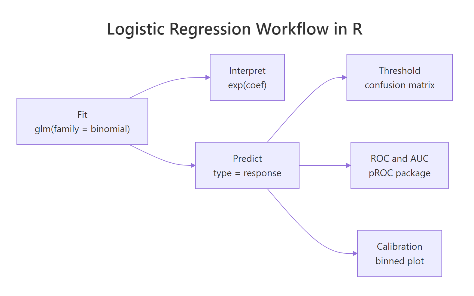
Figure 3: The full fit → interpret → predict → evaluate workflow.
| Step | R idiom | What you get |
|---|---|---|
| Fit | glm(y ~ ..., family = binomial, data = d) |
Model with log-odds coefficients |
| Interpret | broom::tidy(fit, exponentiate = TRUE, conf.int = TRUE) |
Odds ratios with 95% CIs |
| Predict | predict(fit, type = "response") |
Probabilities in [0, 1] |
| Classify | ifelse(probs > threshold, 1, 0) + table() |
Confusion matrix |
| Rank-evaluate | pROC::roc() + auc() + ci.auc() |
ROC curve, AUC, CI |
| Calibrate | Bin predictions, compare mean predicted vs mean actual | Honest probabilities check |
| Overall fit | 1 - fit$deviance / fit$null.deviance |
McFadden pseudo-R² |
Three habits will keep you out of trouble. Coefficients live on the log-odds scale, so always exponentiate before reading them as effect sizes. AUC measures ranking, not calibration, so check both whenever the probabilities themselves matter downstream. And training-set numbers always look better than reality; move to held-out data or cross-validation before you ship anything.
References
- R Core Team, generalised linear models:
?glmdocumentation. Link - James, G., Witten, D., Hastie, T., Tibshirani, R., An Introduction to Statistical Learning, 2nd Edition. Chapter 4: Classification. Link
- Robin, X. et al., pROC: an open-source package for R and S+ to analyze and compare ROC curves. BMC Bioinformatics (2011). Link
- Robinson, D., Hayes, A., Couch, S.,
broom::tidy.glmreference. Link - Hosmer, D. W., Lemeshow, S., Sturdivant, R. X., Applied Logistic Regression, 3rd Edition. Wiley (2013). Link
- Harrell, F., Regression Modeling Strategies, 2nd Edition. Springer (2015). Link
- Steyerberg, E. W., Clinical Prediction Models, 2nd Edition. Springer (2019), chapter on calibration. Link
Continue Learning
- Linear Regression in R, the continuous-outcome sibling that motivates the move to glm.
- Regression Diagnostics in R, residuals, leverage, and influence checks that apply to glm objects too.
- Multinomial Regression With R, the multi-class extension when your outcome has more than two categories.
Further Reading
- Beta Regression in R: betareg Package for Proportions & Rates
- Tobit Regression in R: AER Package for Censored Outcomes
- Multinomial Logistic Regression in R: nnet::multinom() Step-by-Step
- Ordinal Logistic Regression in R: MASS::polr() & Proportional Odds
- Probit & Complementary Log-Log in R: Binary Regression Alternatives
- Logistic Regression Exercises in R: 10 Classification Practice Problems, Solved Step-by-Step
- parsnip logistic_reg() in R: Fit Binary Classifiers