Ridge and Lasso in R: How Penalised Regression Shrinks Coefficients and Selects Variables

Ridge and Lasso are penalised linear regressions that add a cost for large coefficients, trading a little bias for a big drop in variance. Ridge shrinks every coefficient smoothly; Lasso forces some to exactly zero, which doubles as automatic variable selection.

What are Ridge and Lasso regression?

Plain linear regression has one failure mode that shows up everywhere: when predictors outnumber observations, or when several predictors carry similar information, the least-squares fit overreacts. Coefficients become huge, signs flip between nearly identical datasets, and test predictions are worse than the training numbers promised. Ridge and Lasso fix this by adding a penalty on the size of the coefficients. Fit the same model with glmnet and the wild swings disappear.

Here is a first Lasso fit on the classic Boston housing data. Watch how some coefficients land exactly on zero.

Lasso has dropped four predictors, zn, indus, age, and rad, setting their coefficients to exactly zero. The nine survivors are the variables the penalty thinks actually carry signal. An ordinary lm() fit on the same data would keep all thirteen with large, noisy estimates.

How do Ridge and Lasso differ in their penalty?

Both methods start from the same ordinary least-squares loss and bolt a penalty on top. The difference is the shape of that penalty, and the shape is what controls everything downstream.

$$\text{OLS:}\quad \min_{\beta} \sum_{i=1}^{n}\bigl(y_i - x_i^\top \beta\bigr)^2$$

$$\text{Ridge:}\quad \min_{\beta} \sum_{i=1}^{n}\bigl(y_i - x_i^\top \beta\bigr)^2 + \lambda \sum_{j=1}^{p} \beta_j^2$$

$$\text{Lasso:}\quad \min_{\beta} \sum_{i=1}^{n}\bigl(y_i - x_i^\top \beta\bigr)^2 + \lambda \sum_{j=1}^{p} |\beta_j|$$

Where:

• $\beta_j$ is the coefficient on predictor $j$
• $\lambda \ge 0$ is the penalty strength (the tuning parameter)
• $p$ is the number of predictors
• $n$ is the number of observations

Ridge squares each coefficient, so its penalty curves smoothly around zero. Lasso uses absolute values, which draw a diamond with sharp corners at the axes, and those corners are why Lasso can set coefficients to exactly zero. Ridge can only push them close.

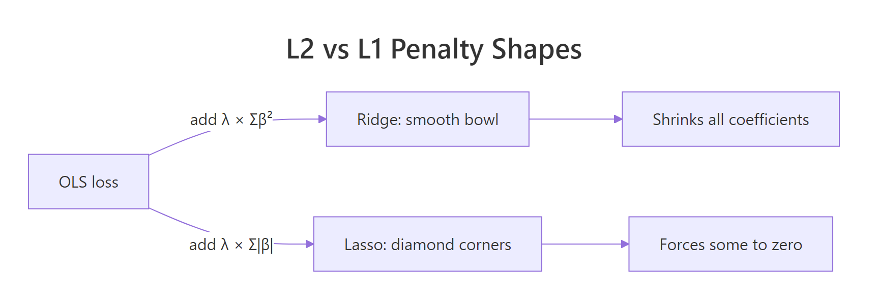
Figure 1: How the L2 and L1 penalties change the same OLS loss.

You can see the difference in one line of R. Fit each method at the same lambda, then count how many coefficients come out zero.

At the same lambda of 0.5, Ridge has zero predictors eliminated and Lasso has four. That single contrast is the whole story of why people reach for Lasso when they want a shorter model and Ridge when they want every predictor kept but tamer.

How do you fit Ridge regression with glmnet?

The glmnet() API has two rules worth burning into memory. First, it does not take a formula: pass a numeric matrix x and a numeric vector y. Second, it fits the full path of lambda values in one call, so one glmnet() object contains 100 models, not just one.

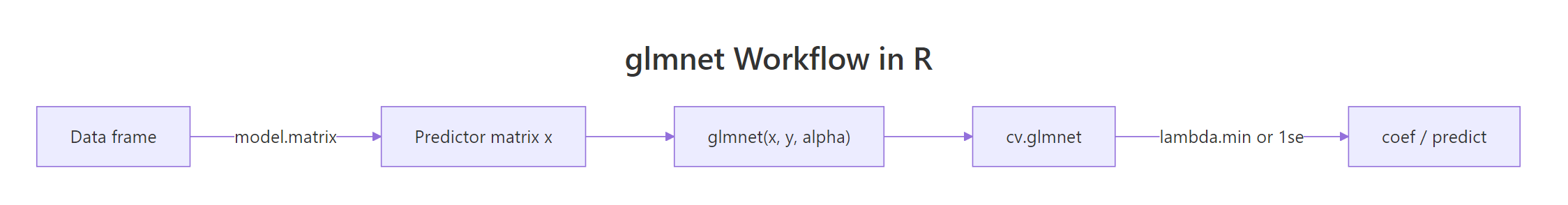
Figure 2: The standard penalised-regression pipeline in R.

Use model.matrix() to turn factor predictors into numeric dummies, drop the intercept column it auto-adds, and then hand the result straight to glmnet with alpha = 0 for Ridge.

Every row is a different lambda. Df counts non-zero coefficients (always 13 for Ridge because it never zeroes any predictor). %Dev is the share of deviance explained, like R-squared. Lambda walks from huge on the left, where every coefficient is crushed to near zero, down to tiny on the right, where the fit approaches plain OLS.

Peek at coefficients at two lambdas to see shrinkage in action.

At s = 0.01 the Ridge coefficients look similar to what lm() would give, just slightly tamed. At s = 100 every coefficient is squeezed close to zero, and the intercept carries most of the prediction. Ridge shrinks proportionally, so the order of importance of predictors stays roughly the same.

How do you fit Lasso regression and select variables?

Flip alpha = 0 to alpha = 1 and glmnet becomes Lasso. The fit returns the same kind of object, but now Df changes as lambda moves, because Lasso can zero predictors out one by one.

Walk the columns left to right. At a large lambda only rm (rooms per dwelling) and lstat (low-income population share) survive, which the housing literature has long called the two dominant predictors of median home value. As lambda shrinks, more variables re-enter in rough order of importance. That ordered entry is why the Lasso path is sometimes called a variable selection path.

Pull the names of non-zero predictors at a single lambda with one which() call.

Nine predictors plus the intercept: glmnet has done model selection and coefficient estimation in a single pass. No p-value forward-selection, no AIC search, no multi-step pipeline.

How do you choose lambda with cross-validation?

Picking lambda by eye is guesswork. cv.glmnet() runs K-fold cross-validation across the lambda path and returns the value that minimises out-of-sample error.

cv.glmnet gives you two lambdas. lambda.min is the value with the lowest cross-validated error. lambda.1se is the largest lambda whose CV error is still within one standard error of the minimum, a more conservative choice that tends to produce simpler models and generalises better on noisy data.

Compare coefficients at both picks to see the trade-off.

lambda.min keeps ten predictors with full-strength coefficients. lambda.1se keeps only six and shrinks them more aggressively. On unseen data the simpler 1se model often predicts better despite fitting worse in training, because it is less tuned to the noise in the training sample.

When should you use Ridge, Lasso, or Elastic Net?

Three penalties, one decision. The right choice depends on what you want the final model to do: keep every predictor and tame them, pick a short list, or handle correlated groups gracefully.

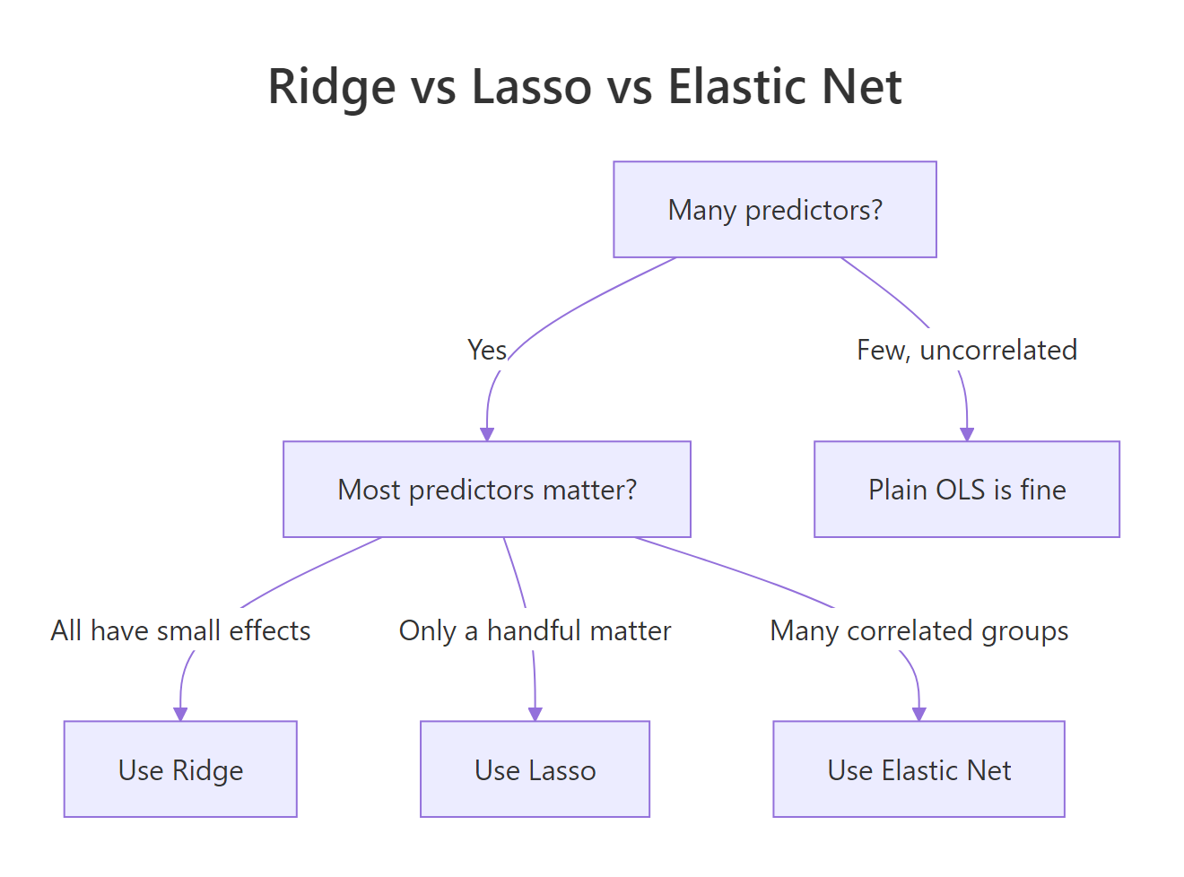
Figure 3: Quick decision tree for picking a penalty.

Fit Elastic Net with alpha = 0.5 and line its error up against the other two.

Elastic Net edges out both Ridge and Lasso on this Boston split, which is typical when a few predictors (here rm and lstat) dominate but a handful of weaker correlated predictors still carry signal.

Finally, predictions. Use predict() with s set to either the lambda name or a numeric value.

All three land close to each other and slightly over the actual value of 24, which is what you would expect for a model that has not seen this exact row but has learned its broader neighbourhood.

Practice Exercises

Each capstone exercise combines several ideas from above. Use distinct variable names so you do not overwrite the tutorial session.

Exercise 1: Lasso variable list at a target sparsity

Fit Lasso on the Boston matrix. Find the lambda on lasso_fit$lambda where exactly six predictors have non-zero coefficients (not counting the intercept). Save the predictor names to my_six.

Exercise 2: Ridge vs OLS on correlated predictors

Simulate 100 rows where x1 and x2 are 0.95 correlated and y = 3*x1 + 3*x2 + rnorm(100). Fit lm() and cv.glmnet(alpha = 0). Save both x1 coefficients side by side to my_results.

Exercise 3: Hold-out RMSE of Ridge vs Lasso

Split Boston 70/30. Fit Ridge and Lasso on the 70% with cv.glmnet. Predict on the 30%. Compute RMSE for each and save both to a named vector my_rmse.

Complete Example

Put every step into one end-to-end workflow on a new simulated dataset with a known sparse signal. Only the first five predictors carry true effect; the next fifteen are pure noise. A good Lasso should find that out.

Lasso recovered the five true predictors and dropped all fifteen noise predictors. The RMSE is close to the irreducible noise standard deviation of 1, meaning the model is almost as good as the oracle. That clean recovery is the reason Lasso is the default first move when you suspect most of your predictors carry nothing.

Summary

Key moves to remember:

1. Build a numeric matrix with model.matrix(formula, data)[, -1].
2. Fit the path with glmnet(x, y, alpha = α) and the CV with cv.glmnet().
3. Pick lambda from cv_fit$lambda.min (best fit) or $lambda.1se (robust fit).
4. Pull coefficients with coef(fit, s = "lambda.min") and predictions with predict(fit, newx = ..., s = ...).
5. set.seed() before any cv.glmnet() call so folds are reproducible.

References

1. glmnet package documentation. Stanford Statistics. Link
2. Hastie, T., Tibshirani, R., Friedman, J. The Elements of Statistical Learning, 2nd ed. Chapter 3.4: Shrinkage Methods. Link
3. Tibshirani, R. Regression Shrinkage and Selection via the Lasso. JRSS Series B (1996). Link
4. Hoerl, A. E., Kennard, R. W. Ridge Regression: Biased Estimation for Nonorthogonal Problems. Technometrics (1970).
5. Zou, H., Hastie, T. Regularization and Variable Selection via the Elastic Net. JRSS Series B (2005). Link
6. James, G., Witten, D., Hastie, T., Tibshirani, R. An Introduction to Statistical Learning, 2nd ed. Chapter 6.2: Shrinkage Methods. Link
7. glmnet CRAN reference manual. Link

Continue Learning

• Linear Regression is the OLS baseline that Ridge and Lasso improve on. Understanding the unpenalised fit makes the shrinkage story concrete.
• Multicollinearity in R covers the problem Ridge was invented to solve. Read it if your regression coefficients flip signs or have large standard errors.
• Variable Selection and Importance With R surveys alternatives to Lasso for picking predictors, including stepwise methods and random-forest importance.