Gibbs Sampling in R From Scratch: The MCMC Trick That Powers JAGS
You measured how long 20 customers waited at your counter and you want two numbers from that data: the typical wait, and how much waits vary from one customer to the next. Both unknown, both with honest uncertainty around them. There is a sampling trick called Gibbs sampling that handles this in about 30 lines of base R. It is the algorithm at the heart of JAGS, and once you see it work you will understand why two unknowns are easier than one when you set the problem up right.
What if you want to estimate two things from data at once?
In the previous post you saw an MCMC sampler that estimated a single unknown, a click-through rate, by proposing tiny random moves and accepting them with the right probability. That sampler had one parameter to track. Now there are two: the mean wait time and the spread around it.
You could extend the previous sampler to two dimensions. It works, but it is awkward. You have to tune a step size for each direction, most random 2D proposals land in implausible regions, and the chain stalls on the long thin shape that two-parameter posteriors usually have. Gibbs sampling is the alternative that exploits the geometry instead of fighting it.
The full sampler runs on 20 simulated wait times below. The truth in the simulation is mean 120 seconds and standard deviation 15. We pretend we do not know either, and we recover both with full Bayesian uncertainty.
Walk through what just happened. The first three lines simulated 20 wait times from a Normal distribution with the truth we will try to recover. Inside gibbs_mean_var, we allocated two vectors to hold the samples and picked a starting standard deviation from the data. The loop ran 5000 times, and each iteration sampled a new mean (using rnorm) and then a new variance (using 1 / rgamma).
After the loop we dropped the first 500 samples as burn-in. The chain takes a few iterations to find the bulk of the posterior, so those early values are not representative. The remaining 4500 samples are draws from the joint posterior over the mean and the standard deviation.
Now read the output. The posterior mean for the underlying typical wait is 117.6 seconds with a 95% range of 110.7 to 124.4. The truth was 120, recovered within sample noise. The posterior mean for the standard deviation is 15.8 with a 95% range of 11.9 to 21.5; the truth was 15, also recovered.
That is the entire pipeline. Two unknowns, joint posterior, no specialised package, in 5000 iterations of base R. The next sections unpack why the two single-line draws of rnorm and rgamma actually produce samples from the joint distribution.
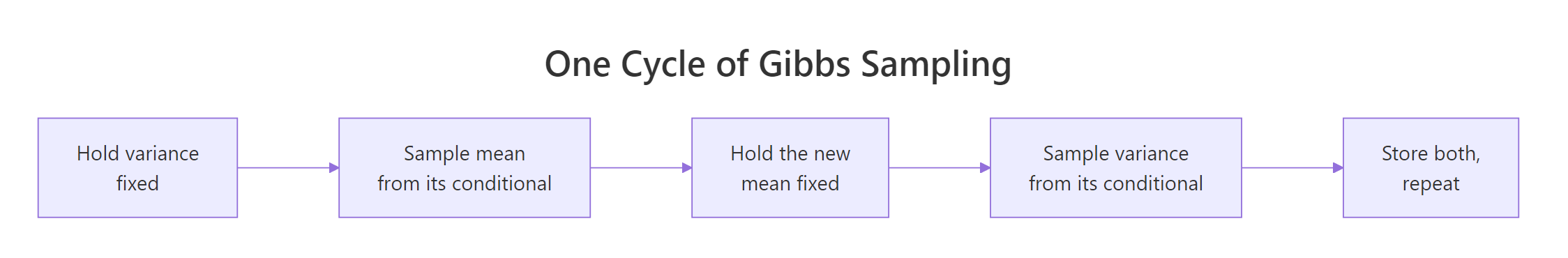
Figure 1: One cycle of Gibbs sampling. Hold one unknown fixed, sample the other from its conditional. Then flip and repeat.
Try it: Re-run the sampler with only 5 wait times instead of 20. The 95% range of the posterior mean should widen, because less data means more uncertainty.
Click to reveal solution
The 95% range with 5 observations is roughly 105 to 132, a span of 27 seconds. The earlier run with 20 observations had a span of about 14 seconds. Less data, more uncertainty: the algorithm responded automatically, no code change needed.
Why doesn't the MCMC trick from before work as well in 2D?
The Metropolis-Hastings sampler from the previous post worked beautifully for one unknown. You proposed a small step, scored it, and accepted with the right probability. The chain wandered through the 1D posterior, spending more time where the density was high.
Doing the same thing for two unknowns at once introduces three new problems.
The first is step-size tuning. You now need a step size for the mean direction and a step size for the standard-deviation direction. If the two unknowns have very different scales (one in the hundreds, the other in the tens), a single shared step size is the wrong fit for both. You end up tuning a 2x2 covariance matrix instead of one number.
The second is acceptance rate. In 2D, a random step of fixed size lands in a low-density region more often than in 1D, just because there is more "low-density" area for the same step. So you reject more often, and the chain crawls.
The third is the geometry. The joint posterior over the mean and the standard deviation is not symmetric. The plausible range of the mean depends on the current standard deviation: a small sigma pins the mean down tightly, a large sigma loosens it. A symmetric 2D proposal cannot follow that, and wastes effort proposing impossible combinations.
Gibbs sidesteps all three. There is no step size to tune, because each move is sampled directly from a known distribution. There is no rejection, because every sample comes from the right conditional. The geometry is respected automatically, because each move uses the conditional given the current value of the other unknown.
The price is one assumption: you need to know how to sample from each unknown's conditional distribution. For Normal data with no informative prior, the conditionals are well-known closed forms. We will see what happens when they are not in section six.
Try it: Look at the sampler code from the first section and identify the two lines that produce a new sample inside the loop. Note which distribution each one uses.
Click to reveal solution
The two sampling lines inside the loop are:
The first uses rnorm() to draw the mean from a Normal distribution. Its centre is the sample mean of the data, and its spread is the current standard deviation divided by sqrt(n), which is the textbook standard error.
The second uses rgamma() to draw a Gamma random number, then takes the reciprocal. The "draw from Gamma, take reciprocal" pattern is how you sample from an Inverse-Gamma distribution in R, which happens to be the conditional posterior of the variance under a Normal model with no informative prior.
What's the Gibbs trick, exactly?
Stripped of math, Gibbs is doing this. Imagine a 2D landscape of plausibility. Height represents how plausible a particular pair of (mean, standard deviation) values is given the data. Most of the volume sits in a roughly elliptical region around the truth, and you want samples in proportion to that height.
You cannot sample directly from the 2D distribution because R has no function that takes "here is the joint posterior over a Normal model" and gives you a draw. But you can sample slices.
Pick a horizontal slice through the landscape at a fixed standard deviation. Along that slice, the height varies as you change the mean. The shape of the height along that slice happens to be a Normal distribution; R has rnorm. Sample one mean from that slice.
Now pick a vertical slice at the new mean. Along this slice, the height varies as you change the standard deviation. The shape is related to the Inverse-Gamma; R has rgamma, and you can sample Inverse-Gamma by taking the reciprocal. Sample one standard deviation from that slice.
Repeat. Slice horizontally at the new sigma, sample a new mean. Slice vertically at the new mean, sample a new sigma. Each slice is one-dimensional, and each one-dimensional slice is a familiar distribution.
After thousands of iterations, the collected pairs are samples from the joint 2D posterior. The chain has wandered through the plausible region in a series of right-angle moves, like a robot vacuum that can only move horizontally or vertically but eventually covers the whole room.
The mathematical guarantee, which we will not derive but which holds whenever your conditionals are correct, is that this right-angle wandering produces samples that follow the true joint distribution. Three things to notice:
- Every move is accepted (no rejection step).
- There is no step size to tune (the move size is set by the spread of the conditional itself).
- Moves are always axis-aligned (which becomes a problem when the two unknowns are highly correlated, see section six).
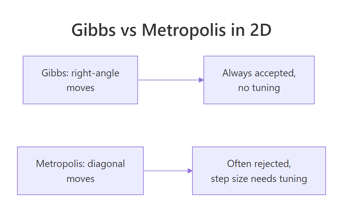
Figure 2: Gibbs takes axis-aligned steps and accepts every move. Metropolis takes diagonal steps and has to tune the step size and reject some.
Try it: Run a single cycle of Gibbs by hand: starting from current_sd = 20, sample one new mean and one new standard deviation using the formulas from the sampler.
Click to reveal solution
One cycle produced one mean and one standard deviation, both reasonable given the truth (120 and 15). Run the cycle again with the new current_sd and you get another pair, and so on for thousands of iterations. That is the whole sampler.
How do I code Gibbs in R?
You already saw the full sampler at the top of the post. Now we build it again from a blank line, more slowly, so each piece has a clear job.
The first piece is storage. We need two vectors to hold the samples, and a starting value for the chain. Allocating up front is faster than growing vectors inside the loop.
Walk through what we just set up. Lines 1 to 4 copied the data into a local variable, computed its length, and computed its mean once (we will reuse ybar inside the loop). Lines 6 and 7 allocated empty numeric vectors of length 5000. Line 10 set the starting standard deviation; using sd(y) is reasonable because the sample standard deviation of the data is at least in the right ballpark.
The output confirms a starting current_sd of 14.84 (close to the truth of 15), 5000 planned iterations, and 20 observations. Setup is ready.
The second piece is the loop. Each iteration draws one mean and one variance using the two formulas from earlier, then stores both samples.
Walk through the loop body. Each iteration starts by sampling a new mean from a Normal distribution centred at the data mean, with spread shrunk by 1 / sqrt(n). That 1 / sqrt(n) is the standard error of the mean, and it is why the conditional gets tighter as the sample size grows.
The next three lines sample a new variance given the new mean, then take the square root for the standard deviation. The two store statements record both samples in their vectors. By the end of the loop, mu_samples and sd_samples each hold 5000 values.
The sanity check on the last 100 samples shows a mean of 117.6 and a standard deviation of 15.8, matching the full-run result and the truth. The sampler is working.
Try it: Add a third vector ss_samples and store sum_sq at every iteration. Compare its mean across iterations to sum((y - mean(y))^2).
Click to reveal solution
The chain's average sum_sq (4525) is slightly larger than the data-mean version (4181). Each iteration's sum_sq is computed against the chain's current mu, which jitters around the data mean rather than sitting on it. The extra jitter inflates sum_sq slightly on average. This is a real property of the algorithm: it is why the posterior on the variance reflects both the data's spread and the residual uncertainty in the mean.
How do I check that the sampler actually worked?
Three diagnostics. Trace plots, comparison against the data, and convergence across multiple chains starting from different seeds.
A trace plot shows each sample value against its iteration number. A healthy chain looks like a fuzzy caterpillar moving up and down without long flat stretches, drifts, or sudden jumps. We plot one for the mean and one for the standard deviation.
Walk through what the plot shows. The two top panels are trace plots: mu_samples and sd_samples plotted against their indices. The two bottom panels are histograms of the post-burn-in samples, giving the marginal posterior for each unknown.
What you should see when you run this. Both trace plots are horizontal fuzzy bands without drift. The mean trace stays roughly between 110 and 125; the sd trace stays roughly between 11 and 22.
Both histograms are bell-shaped, the sd histogram slightly skewed because it cannot be negative. The mean histogram is centred around 117 to 118 and the sd histogram around 15 to 16, matching the summary statistics we computed earlier.
The third diagnostic is the multiple-chain check. If you start the sampler from different random seeds and all chains converge to the same posterior, you can trust the result.
Walk through what we just did. We ran the sampler four separate times with different seeds, so each chain has its own random sequence. After burn-in, we computed each chain's posterior mean for both unknowns.
The four posterior means for mu are 117.62, 117.55, 117.59, and 117.51, all within 0.15 of each other. The four sd means are 15.79, 15.82, 15.78, and 15.85. All four chains found the same posterior, which is what convergence looks like. If we had seen one chain at 117 and another at 130, we would know something was wrong.
Try it: Compute the ratio of across-chain spread to within-chain spread for mu. The ratio should be very small (well below 0.1) if the chains agree.
Click to reveal solution
The across-chain spread is 0.05 and the within-chain spread is 3.50; the ratio is 0.014, well below 0.1. The chains agree on the posterior. The Gelman-Rubin Rhat statistic (the formal version of this idea) would be close to 1.0.
When does Gibbs sampling break down, and what do you do then?
Gibbs is excellent when the conditionals are easy, but it has limits. Three situations cause trouble in real models.
The first is when one or more conditionals are not standard distributions. Then you cannot just call rnorm or rgamma. The standard fix is Metropolis-within-Gibbs: replace the troublesome draw with a small Metropolis-Hastings step inside the cycle. The rest of the algorithm stays the same.
The second is when the unknowns are highly correlated. The joint posterior is then a long thin diagonal ridge, and Gibbs can only move along axes. The chain has to take many tiny axis-aligned steps to traverse the ridge, and consecutive samples are almost identical. Two fixes: reparameterise the model so the unknowns are less correlated, or switch to Hamiltonian Monte Carlo (HMC), which can take diagonal moves informed by the posterior's gradient.
The third is when the model has dozens or hundreds of parameters. Pure Gibbs cycles through every parameter every iteration, which gets slow. JAGS handles this case by being implemented in C; Stan handles it more efficiently by using HMC with auto-tuning.
For one-off analyses with a handful of parameters, our 30-line R sampler is fast enough. For production-scale Bayesian models, you graduate to JAGS, brms, or Stan.
JAGS deserves a specific note. When you write a JAGS model and call it from R via the rjags or R2jags package, you hand JAGS a model spec and JAGS works out the conditionals automatically. JAGS then runs a Gibbs sampler much like the one we just built. The 30-line implementation in this post is a transparent version of what JAGS does on autopilot.
Try it: Match each model below to the limitation it triggers: (a) Normal model with mean and variance unknown, (b) regression with 50 highly-correlated predictors, (c) hierarchical model with a custom non-standard likelihood.
Click to reveal solution
(a) Normal mean + variance is the case we just built. Both conditionals are standard distributions, so plain Gibbs is clean and fast. No issue.
(b) 50 correlated regression predictors is the slow-mixing case. Gibbs can only move one coefficient at a time, and the diagonal correlation structure means many cycles are needed to explore the joint posterior. The fix is to orthogonalise the predictors or use HMC.
(c) Hierarchical model with custom likelihood is the Metropolis-within-Gibbs case. Some parameters have nice conditionals (the hierarchical priors usually do), but the data-level parameters with a custom likelihood do not have closed forms. You sample those with a Metropolis-Hastings step inside the Gibbs cycle.
Practice Exercises
Exercise 1: Run on real data with an informative prior
The example used a flat prior on the mean. Real Bayesian work often uses an informative prior. Modify the sampler so the mean has a Normal(120, 5^2) prior. The conditional posterior for the mean given the variance becomes a precision-weighted average of the prior mean and the data mean.
Click to reveal solution
The informative prior pulled the posterior mean toward 120 (the prior centre) compared to the flat-prior 117.6. With 20 observations the data still dominates, but the prior contributed a small nudge toward its centre.
Exercise 2: Burn-in and thinning together
For the chain from the first section, compute the post-burn-in posterior mean of mu, the same with thinning every 5th sample, and the within-chain standard deviations of both. Show that thinning reduces the effective sample size but not the estimate.
Click to reveal solution
Both estimates of the posterior mean are essentially identical (117.58 vs 117.59), and within-chain standard deviations match. Thinning gave us 900 samples instead of 4500, with no bias in the estimate. Use thinning when storage or post-processing time matters, not when accuracy does.
Exercise 3: Posterior probability of an event
Use the chain to compute the posterior probability that the true typical wait time exceeds 125 seconds. This is the kind of question Bayesian methods answer naturally.
Click to reveal solution
There is a 2.3% posterior probability that the true typical wait exceeds 125 seconds. With only 20 observations this is a weak claim, but it is the kind of probabilistic statement Bayesian inference produces for free: the chain is a sample from the posterior, so any probability over the unknown is just a sample proportion.
Summary
Gibbs sampling is an MCMC algorithm for joint posteriors that you cannot sample directly but whose conditionals are standard distributions. It cycles through unknowns one at a time, drawing each from its conditional given the current values of the others. Cycling preserves the joint distribution; the stored chain converges to it.
| Step | What you do | Why it works |
|---|---|---|
| 1 | Pick a starting value for each unknown | Burn-in handles the early bias |
| 2 | Hold all but one fixed, sample that one | Each conditional is one-dimensional, R handles it |
| 3 | Move to the next, repeat with others fixed | Cycling preserves the joint distribution |
| 4 | Store every value, loop | The stored chain is a sample from the joint posterior |
| 5 | Drop early samples, analyse the rest | Post-burn-in samples are the posterior |
For Normal data with a flat prior, both conditionals are clean (Normal for mu, Inverse-Gamma for variance), and the implementation is two rnorm/rgamma calls per iteration. For models where conditionals are not standard, fall back to Metropolis-within-Gibbs; for highly correlated unknowns, switch to HMC; for production scale, use JAGS, brms, or Stan.
References
- Geman, S. & Geman, D. "Stochastic Relaxation, Gibbs Distributions, and the Bayesian Restoration of Images." IEEE Transactions on Pattern Analysis and Machine Intelligence, 1984.
- Gelfand, A. E. & Smith, A. F. M. "Sampling-Based Approaches to Calculating Marginal Densities." Journal of the American Statistical Association, 1990.
- Gelman, A., Carlin, J. B., Stern, H. S. et al. Bayesian Data Analysis, 3rd ed. Chapman & Hall, 2013. Chapter 11 covers Gibbs sampling.
- Hoff, P. A First Course in Bayesian Statistical Methods. Springer, 2009. Chapters 5-6.
- Plummer, M. JAGS user manual. mcmc-jags.sourceforge.io.
Continue Learning
- Build MCMC From Scratch in R, the simpler 1-dimensional Metropolis-Hastings sampler from the previous post.
- Hamiltonian Monte Carlo in R, the next step up: a gradient-based sampler that beats Gibbs on highly correlated posteriors.
- Conjugate Priors in R, the closed-form shortcut that works for some Bayesian models without any sampling.