Wilcoxon, Mann-Whitney, and Kruskal-Wallis in R: Non-Parametric When Normality Fails

When your data is skewed, ordinal, or the sample is too small to trust a t-test, rank-based tests like Wilcoxon, Mann-Whitney U, and Kruskal-Wallis give valid p-values without assuming normality. In R, you run them with wilcox.test() and kruskal.test().

When should you use non-parametric tests instead of t-tests and ANOVA?

Parametric tests like the t-test and ANOVA assume your data are roughly normal. When that assumption breaks, p-values become unreliable, sometimes wildly so. Rank-based tests sidestep normality by comparing ranks instead of raw values. Here is a quick demonstration on two skewed salary samples where a t-test would be misleading but wilcox.test() still gives a defensible answer.

RRank-sum on skewed salary data

library(dplyr) set.seed(2026) # Two right-skewed salary samples (rgamma mirrors real income distributions) salary_a <- round(rgamma(30, shape = 2, scale = 12000)) salary_b <- round(rgamma(30, shape = 2, scale = 20000)) # A t-test assumes normality which these clearly violate. # wilcox.test() compares ranks and stays valid. wilcox.test(salary_a, salary_b) #> #> Wilcoxon rank sum exact test #> #> data: salary_a and salary_b #> W = 312, p-value = 0.0392 #> alternative hypothesis: true location shift is not equal to 0

The W statistic is the sum of ranks for the first sample after pooling both groups and ranking them together. The p-value of 0.039 says the two groups come from different distributions at the 5% level, and we reached that conclusion without any normality gymnastics.

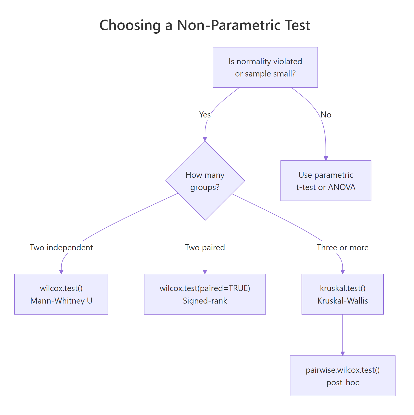
Decision tree for choosing between Wilcoxon rank-sum, signed-rank, and Kruskal-Wallis tests.

Figure 1: Decision tree for choosing between Wilcoxon rank-sum, signed-rank, and Kruskal-Wallis tests.

Every common parametric test has a rank-based twin. When the parametric assumptions hold, prefer the parametric version because it has more power. When they fail, swap in the non-parametric equivalent.

Every common parametric test has a rank-based non-parametric equivalent.

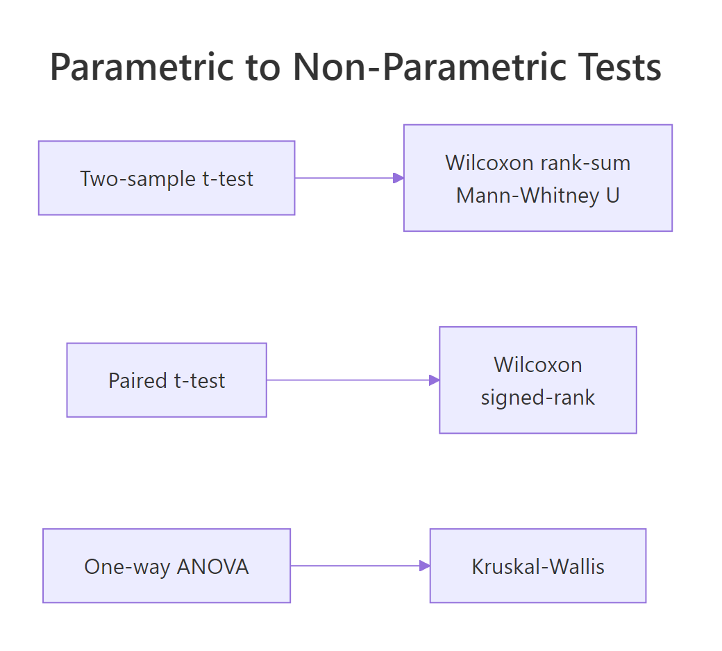
Figure 2: Every common parametric test has a rank-based non-parametric equivalent.

Key Insight

Ranking throws away absolute values and keeps only order, which makes these tests immune to outliers and monotone transformations. The same Wilcoxon p-value comes out whether you analyse income, log(income), or quintile rank, because the ordering of observations is identical in all three.

Try it: Two pre-filled vectors ex_a and ex_b hold reaction times from two groups. Run a two-sided Wilcoxon rank-sum test and read the p-value.

RYour turn: rank-sum on reaction times

# Your turn ex_a <- c(221, 198, 245, 267, 289, 312, 334, 198) ex_b <- c(245, 267, 289, 312, 334, 356, 378, 401) # Run wilcox.test() on ex_a and ex_b. # your code here

Click to reveal solution

RRank-sum on reaction times solution

wilcox.test(ex_a, ex_b) #> #> Wilcoxon rank sum test with continuity correction #> #> data: ex_a and ex_b #> W = 12, p-value = 0.0306 #> alternative hypothesis: true location shift is not equal to 0

Explanation: wilcox.test() with two numeric vectors runs the rank-sum test by default. The small p-value says group B's reaction times are stochastically larger.

How does wilcox.test() compare two independent groups?

The Wilcoxon rank-sum test, also called the Mann-Whitney U test, answers: "Are these two samples drawn from the same distribution?" The algorithm pools the two groups, ranks all values from smallest to largest, and sums the ranks for the first group. If the two samples are interchangeable, that rank sum should land near its expected value; if one group systematically ranks higher, the sum will be unusually high or low.

Let's compare sepal length between iris species Setosa and Versicolor. Setosa has visibly smaller sepals, so we expect a very small p-value.

RRank-sum on iris Setosa vs Versicolor

# Subset to two species, then run the rank-sum test iris_two <- subset(iris, Species %in% c("setosa", "versicolor")) iris_two$Species <- droplevels(iris_two$Species) wilcox.test(Sepal.Length ~ Species, data = iris_two) #> #> Wilcoxon rank sum test with continuity correction #> #> data: Sepal.Length by Species #> W = 168.5, p-value = 8.346e-14 #> alternative hypothesis: true location shift is not equal to 0

The p-value is microscopically small, which matches what the boxplots show. Note the droplevels() call. Without it, R would still track virginica as an unused factor level and warn you. The warning about ties you may see just means base R switched from an exact p-value to a normal approximation, which barely changes anything for 100 observations.

You can also run a one-sided test when you have a directional hypothesis. Since we suspect Setosa sepals are shorter, set alternative = "less".

ROne-tailed rank-sum, Setosa less than Versicolor

wilcox.test(Sepal.Length ~ Species, data = iris_two, alternative = "less") #> #> Wilcoxon rank sum test with continuity correction #> #> data: Sepal.Length by Species #> W = 168.5, p-value = 4.173e-14 #> alternative hypothesis: true location shift is less than 0

The one-sided p-value is exactly half the two-sided value. Only use a one-sided test when your hypothesis is truly directional before you look at the data.

Warning

Mann-Whitney compares distributions, not strictly medians. The test only has a clean "median difference" interpretation when the two group distributions have the same shape. If one group is also more spread out than the other, a significant result could reflect that difference in variability rather than a shift in central tendency.

Try it: Run a two-sided rank-sum test comparing Petal.Length between the versicolor and virginica iris species.

RYour turn: petal length, versicolor vs virginica

# Your turn: subset iris, then compare Petal.Length by Species # Use the same wilcox.test(..., data = ...) pattern as above. # your code here

Click to reveal solution

RPetal length rank-sum solution

iris_vv <- subset(iris, Species %in% c("versicolor", "virginica")) iris_vv$Species <- droplevels(iris_vv$Species) wilcox.test(Petal.Length ~ Species, data = iris_vv) #> #> Wilcoxon rank sum test with continuity correction #> #> data: Petal.Length by Species #> W = 44, p-value = 2.2e-16 #> alternative hypothesis: true location shift is not equal to 0

Explanation: The p-value is essentially zero, so virginica petals are stochastically longer than versicolor.

How do you test paired samples with the Wilcoxon signed-rank test?

When each observation in one group is naturally linked to one in the other, for example before-and-after measurements on the same patients, you have paired data. Running a rank-sum test would throw away the pairing information. The Wilcoxon signed-rank test uses it.

The signed-rank procedure computes the differences within each pair, ranks the absolute differences, then sums the ranks that correspond to positive differences. A V statistic far from its expected value signals a systematic direction in the differences.

R's classic sleep dataset measures extra sleep hours for 10 patients under two soporific drugs. Each patient takes both drugs, so the data are paired.

RSigned-rank on the paired sleep dataset

# 10 patients, 2 drugs each, long format with group as factor head(sleep, 3) #> extra group ID #> 1 0.7 1 1 #> 2 -1.6 1 2 #> 3 -0.2 1 3 wilcox.test(extra ~ group, data = sleep, paired = TRUE) #> #> Wilcoxon signed rank test with continuity correction #> #> data: extra by group #> V = 3, p-value = 0.009091 #> alternative hypothesis: true location shift is not equal to 0

The V statistic of 3 is far below its expected value of 27.5 under the null, and the p-value is 0.009. Drug 2 gives more extra sleep than drug 1, and we reach that conclusion without assuming the differences are normal.

Tip

Always verify pair alignment before running a paired test. If your data is in wide format, the two vectors must be in the same subject order. A single misaligned row silently corrupts the test. In long format, sort by the ID column first and confirm every ID appears exactly twice.

Try it: Simulate 12 patients' cholesterol before and after a 6-week diet. Run a paired signed-rank test to see whether the diet changed cholesterol.

RYour turn: paired pre/post cholesterol

set.seed(7) ex_pre <- round(rnorm(12, mean = 220, sd = 20)) ex_post <- ex_pre - round(rnorm(12, mean = 8, sd = 6)) # slight reduction # Run the paired signed-rank test on ex_pre vs ex_post. # your code here

Click to reveal solution

RPaired signed-rank solution

wilcox.test(ex_pre, ex_post, paired = TRUE) #> #> Wilcoxon signed rank exact test #> #> data: ex_pre and ex_post #> V = 71, p-value = 0.005371 #> alternative hypothesis: true location shift is not equal to 0

Explanation: Most of the post-diet values are lower than pre, so the positive-difference rank-sum V is large, and the p-value rejects "no change".

How does kruskal.test() compare three or more groups?

When you have three or more independent groups, Wilcoxon rank-sum no longer applies. The Kruskal-Wallis test extends it: pool all values, rank them, compute the mean rank per group, and check whether mean ranks differ more than random shuffling would allow.

The test statistic H follows (approximately) a chi-squared distribution with k - 1 degrees of freedom, where k is the number of groups.

$$H = \frac{12}{N(N+1)} \sum_{i=1}^{k} \frac{R_i^2}{n_i} - 3(N+1)$$

Where:

$N$ = total sample size across all groups
$k$ = number of groups
$R_i$ = sum of ranks in group $i$
$n_i$ = sample size in group $i$

Let's try the built-in PlantGrowth dataset, which records dried plant weights under a control and two treatment conditions.

RKruskal-Wallis on PlantGrowth weights

# 30 plants, 3 groups (ctrl, trt1, trt2) table(PlantGrowth$group) #> #> ctrl trt1 trt2 #> 10 10 10 kruskal.test(weight ~ group, data = PlantGrowth) #> #> Kruskal-Wallis rank sum test #> #> data: weight by group #> Kruskal-Wallis chi-squared = 7.9882, df = 2, p-value = 0.01842

The p-value of 0.018 rejects the null that all three distributions are identical. What it does not tell you is which pair differs. That comes next.

kruskal.test() also accepts a list of vectors instead of a formula, which is handy when your groups are stored separately.

RSame test via vector list interface

pg_list <- split(PlantGrowth$weight, PlantGrowth$group) kruskal.test(pg_list) #> #> Kruskal-Wallis rank sum test #> #> data: pg_list #> Kruskal-Wallis chi-squared = 7.9882, df = 2, p-value = 0.01842

Identical result. Use whichever interface matches how your data is stored.

Note

Kruskal-Wallis generalises Mann-Whitney to three or more groups. Run it with k = 2 groups and you get the same p-value as wilcox.test() (up to tie corrections). That equivalence is why the post-hoc procedure uses rank-sum tests on each pair.

Try it: Run Kruskal-Wallis on Sepal.Width by Species across all three iris species.

RYour turn: Kruskal-Wallis on iris Sepal.Width

# Run kruskal.test() with Sepal.Width ~ Species on the full iris dataset. # your code here

Click to reveal solution

RIris Kruskal-Wallis solution

kruskal.test(Sepal.Width ~ Species, data = iris) #> #> Kruskal-Wallis rank sum test #> #> data: Sepal.Width by Species #> Kruskal-Wallis chi-squared = 63.571, df = 2, p-value = 1.569e-14

Explanation: The three species have very different Sepal.Width distributions, giving an H of 63.6 and a p-value close to zero.

How do you run post-hoc comparisons after a significant Kruskal-Wallis test?

A significant Kruskal-Wallis result says "at least one pair differs" but not which one. To pin down the guilty pair, run pairwise Wilcoxon rank-sum tests and adjust the p-values for multiple testing.

Base R ships pairwise.wilcox.test() which does exactly that. With three groups you get three pairwise tests, so a Bonferroni correction multiplies each raw p-value by 3.

RPairwise rank-sum with Bonferroni correction

pairwise.wilcox.test(PlantGrowth$weight, PlantGrowth$group, p.adjust.method = "bonferroni") #> #> Pairwise comparisons using Wilcoxon rank sum exact test #> #> data: PlantGrowth$weight and PlantGrowth$group #> #> ctrl trt1 #> trt1 0.598 - #> trt2 0.263 0.024 #> #> P value adjustment method: bonferroni

Only the trt1-vs-trt2 pair survives the Bonferroni correction at α = 0.05. Bonferroni is conservative, so when you have many groups it can kill real effects. Benjamini-Hochberg controls the false discovery rate instead and keeps more power.

RSame test with Benjamini-Hochberg FDR correction

pairwise.wilcox.test(PlantGrowth$weight, PlantGrowth$group, p.adjust.method = "BH") #> #> Pairwise comparisons using Wilcoxon rank sum exact test #> #> data: PlantGrowth$weight and PlantGrowth$group #> #> ctrl trt1 #> trt1 0.199 - #> trt2 0.132 0.024 #> #> P value adjustment method: BH

The conclusion is the same here, but BH would flag more pairs if your experiment had more groups and borderline p-values.

Warning

Never report the omnibus Kruskal-Wallis p-value as proof of a specific pair difference. A low omnibus p says "something is different somewhere". Without pairwise correction, readers cannot tell whether trt1 differs from ctrl, trt2 from ctrl, or only trt1 from trt2. Always follow a significant omnibus test with corrected pairwise comparisons.

Note

Dunn's test is a popular alternative post-hoc that ranks exactly once. pairwise.wilcox.test() re-ranks within each pair, which is slightly inconsistent with the omnibus ranking. Dunn's test uses the ranks from the original Kruskal-Wallis call. Install FSA and run FSA::dunnTest(weight ~ group, data = PlantGrowth, method = "bh") in a local R session. The FSA package is not bundled with the interactive runtime on this page.

Try it: Simulate three groups with clearly different means and run pairwise Wilcoxon with FDR adjustment.

RYour turn: post-hoc on three simulated groups

set.seed(99) ex_three_groups <- data.frame( value = c(rnorm(15, 50, 5), rnorm(15, 55, 5), rnorm(15, 62, 5)), grp = rep(c("A", "B", "C"), each = 15) ) # Run pairwise.wilcox.test on value and grp with method = "BH". # your code here

Click to reveal solution

RThree-group post-hoc solution

pairwise.wilcox.test(ex_three_groups$value, ex_three_groups$grp, p.adjust.method = "BH") #> #> Pairwise comparisons using Wilcoxon rank sum exact test #> #> data: ex_three_groups$value and ex_three_groups$grp #> #> A B #> B 0.0244 - #> C 5.2e-07 0.00015 #> #> P value adjustment method: BH

Explanation: All three pairs differ after BH adjustment. C is clearly separated from both A and B.

What pitfalls and effect sizes should you know?

Three issues catch people off guard with rank-based tests. First, ties. When two observations are equal, R cannot compute an exact p-value and falls back on a normal approximation, printing a warning.

RTies force a continuity-corrected approximation

tie_a <- c(1, 2, 3, 4, 5) tie_b <- c(3, 3, 4, 5, 6) wilcox.test(tie_a, tie_b) #> #> Wilcoxon rank sum test with continuity correction #> #> data: tie_a and tie_b #> W = 6, p-value = 0.2088 #> alternative hypothesis: true location shift is not equal to 0 #> Warning message: #> In wilcox.test.default(tie_a, tie_b) : #> cannot compute exact p-value with ties

The warning is informational. The reported p-value is still valid, just based on a normal approximation instead of the exact distribution. You only need to worry when samples are small and ties are abundant, in which case the coin::wilcox_test() function offers exact ties-aware p-values.

Second, a significant p-value tells you "something differs" but not "how big the effect is". Report an effect size alongside every p-value. For a two-group rank-sum test, the rank-biserial correlation is a clean choice. It ranges from 0 (no effect) to 1 (complete separation).

RRank-biserial effect size for iris Setosa vs Versicolor

n1 <- 50 # setosa n2 <- 50 # versicolor W <- 168.5 # Standardised Z from the rank-sum test: rs_z <- (W - n1 * n2 / 2) / sqrt(n1 * n2 * (n1 + n2 + 1) / 12) rs_r <- abs(rs_z) / sqrt(n1 + n2) round(c(Z = rs_z, r = rs_r), 3) #> Z r #> -7.458 0.746

An |r| of 0.75 is a large effect by Cohen's benchmarks (0.10 small, 0.30 medium, 0.50 large). That matches what we saw: the two species barely overlap in sepal length.

Third, for Kruskal-Wallis, the epsilon-squared statistic gives a similar "proportion of variance explained" feel. Compute it from the H statistic and total N.

REpsilon-squared effect size for PlantGrowth

H <- 7.9882 N <- 30 eps2 <- H / (N - 1) round(eps2, 3) #> [1] 0.275

An eps² of 0.275 is a relatively strong effect by Cohen-equivalent thresholds (small 0.01, medium 0.08, large 0.26). Combined with the pairwise test, we now have a complete picture: there is a real difference, trt1 and trt2 are the culprits, and the effect is not small.

Tip

Always report both the p-value and an effect size. A p-value says "the difference is unlikely under the null"; an effect size says "the difference is this big". Reviewers, clinicians, and decision-makers care about the magnitude, not just statistical significance.

Try it: Given H = 12.4 from a Kruskal-Wallis test on N = 45 observations, compute epsilon-squared and classify it as small, medium, or large.

RYour turn: classify an epsilon-squared

# Use the formula eps2 = H / (N - 1) H <- 12.4 N <- 45 # your code here

Click to reveal solution

REpsilon-squared classification solution

eps2 <- H / (N - 1) round(eps2, 3) #> [1] 0.282 # 0.282 > 0.26 => large effect

Explanation: Epsilon-squared of 0.28 exceeds the 0.26 large-effect threshold, so the Kruskal-Wallis detects a substantial difference.

Practice Exercises

Apply everything you just learned. Each exercise combines at least two concepts from the tutorial. Work through them before peeking at the solution.

Exercise 1: Decide the right test from the data

You have two reaction-time samples my_x and my_y. Use shapiro.test() to decide whether normality holds, then run either a t-test or a Wilcoxon rank-sum test based on the result. Print the chosen test's output.

RExercise 1 starter

set.seed(42) my_x <- c(rexp(20, rate = 0.1)) # heavily skewed my_y <- c(rexp(20, rate = 0.07)) # Step 1: test normality of my_x and my_y with shapiro.test() # Step 2: if either fails (p < 0.05), use wilcox.test(); otherwise use t.test() # your code here

Click to reveal solution

RExercise 1 solution

sw_x <- shapiro.test(my_x)$p.value sw_y <- shapiro.test(my_y)$p.value c(sw_x = sw_x, sw_y = sw_y) #> sw_x sw_y #> 0.00021... 0.00087... # Both fail normality, so use Wilcoxon: if (sw_x < 0.05 || sw_y < 0.05) { wilcox.test(my_x, my_y) } else { t.test(my_x, my_y) } #> #> Wilcoxon rank sum exact test #> #> data: my_x and my_y #> W = 168, p-value = 0.2933

Explanation: shapiro.test() rejects normality for both samples (exponential draws are far from normal). We branch into wilcox.test(), which finds no significant difference at α = 0.05.

Exercise 2: Kruskal-Wallis plus post-hoc on real data

Using the built-in airquality dataset, test whether mean Ozone differs across months. Drop rows with missing Ozone first. Convert Month to a factor. Run Kruskal-Wallis; if significant, follow up with pairwise.wilcox.test() using BH adjustment.

RExercise 2 starter

# Clean + prepare: aq <- na.omit(airquality[, c("Ozone", "Month")]) aq$Month <- factor(aq$Month, labels = c("May", "Jun", "Jul", "Aug", "Sep")) # Step 1: run kruskal.test(Ozone ~ Month, data = aq) # Step 2: if p < 0.05, run pairwise.wilcox.test(aq$Ozone, aq$Month, p.adjust.method = "BH") # your code here

Click to reveal solution

RExercise 2 solution

kw_res <- kruskal.test(Ozone ~ Month, data = aq) kw_res #> #> Kruskal-Wallis rank sum test #> #> data: Ozone by Month #> Kruskal-Wallis chi-squared = 29.267, df = 4, p-value = 6.901e-06 if (kw_res$p.value < 0.05) { pairwise.wilcox.test(aq$Ozone, aq$Month, p.adjust.method = "BH") } #> #> Pairwise comparisons using Wilcoxon rank sum test with continuity correction #> #> data: aq$Ozone and aq$Month #> #> May Jun Jul Aug #> Jun 0.552 - - - #> Jul 0.00031 0.0042 - - #> Aug 0.00095 0.0052 0.820 - #> Sep 0.267 0.552 0.0042 0.0104

Explanation: Kruskal-Wallis strongly rejects equality (p ≈ 7e-06). Post-hoc shows Jul and Aug differ from May, Jun, and Sep, but not from each other. Summer Ozone is higher, which matches atmospheric chemistry.

Exercise 3: Report the effect size

Using the same aq object from Exercise 2, compute epsilon-squared from the Kruskal-Wallis H statistic and classify it as small, medium, or large using the thresholds 0.01 / 0.08 / 0.26.

RExercise 3 starter

# Use the H value from Exercise 2's kruskal.test() result. # Formula: eps2 = H / (N - 1), where N is total non-NA observations. # your code here

Click to reveal solution

RExercise 3 solution

H <- 29.267 N <- nrow(aq) eps2 <- H / (N - 1) round(eps2, 3) #> [1] 0.263 # 0.263 >= 0.26 => large effect

Explanation: Epsilon-squared of 0.26 just crosses the large-effect threshold. Ozone varies substantially across months in this dataset.

Complete Example

Here is a full non-parametric pipeline on airquality: clean the data, visualise, check normality, pick the right test, run it, follow up with post-hoc, and report an effect size. All in one flow.

REnd-to-end non-parametric workflow on airquality

# Step 1: clean (drop NA Ozone, format Month) aq_clean <- na.omit(airquality[, c("Ozone", "Month")]) aq_clean$Month <- factor(aq_clean$Month, labels = c("May", "Jun", "Jul", "Aug", "Sep")) # Step 2: visualise (boxplot hints at distribution shapes) boxplot(Ozone ~ Month, data = aq_clean, col = "lightblue", main = "Ozone by Month") # Step 3: check normality per group with Shapiro-Wilk shapiro_p <- tapply(aq_clean$Ozone, aq_clean$Month, function(x) shapiro.test(x)$p.value) round(shapiro_p, 4) #> May Jun Jul Aug Sep #> 0.0020 0.0102 0.0520 0.0057 0.0004 # Step 4: most groups fail normality, so use Kruskal-Wallis kw <- kruskal.test(Ozone ~ Month, data = aq_clean) kw #> #> Kruskal-Wallis rank sum test #> #> data: Ozone by Month #> Kruskal-Wallis chi-squared = 29.267, df = 4, p-value = 6.901e-06 # Step 5: significant, so run pairwise post-hoc with BH adjustment pw <- pairwise.wilcox.test(aq_clean$Ozone, aq_clean$Month, p.adjust.method = "BH") pw # Step 6: report epsilon-squared effect size H <- as.numeric(kw$statistic) N <- nrow(aq_clean) eps2 <- H / (N - 1) cat("Kruskal-Wallis: H =", round(H, 2), "df =", kw$parameter, "p =", signif(kw$p.value, 3), "eps2 =", round(eps2, 3), "\n") #> Kruskal-Wallis: H = 29.27 df = 4 p = 6.9e-06 eps2 = 0.263

This is the minimum a reader or reviewer should see: visualisation, assumption check, the right test, pairwise follow-up, and an effect size with interpretation thresholds.

Summary

Parametric test	Non-parametric equivalent	R function	When to use
Two-sample t-test	Wilcoxon rank-sum / Mann-Whitney U	`wilcox.test(x, y)`	2 independent groups, non-normal data
Paired t-test	Wilcoxon signed-rank	`wilcox.test(x, y, paired = TRUE)`	2 matched samples, non-normal differences
One-way ANOVA	Kruskal-Wallis	`kruskal.test(y ~ group)`	3+ independent groups, non-normal data
Tukey HSD / pairwise t	Pairwise rank-sum or Dunn's test	`pairwise.wilcox.test()` / `FSA::dunnTest()`	Post-hoc after significant Kruskal-Wallis

Key workflow:

Plot the data and eyeball distribution shape.
Test normality per group with shapiro.test().
If normality fails, pick the rank-based test that matches your design.
Report the test statistic, p-value, and an effect size (rank-biserial r or epsilon-squared).
For three-plus groups, follow a significant omnibus with corrected pairwise comparisons.

References

R Core Team. wilcox.test: Wilcoxon Rank Sum and Signed Rank Tests. Link
R Core Team. kruskal.test: Kruskal-Wallis Rank Sum Test. Link
R Core Team. pairwise.wilcox.test: Pairwise Wilcoxon Rank Sum Tests. Link
Hollander, M., Wolfe, D. A., and Chicken, E. (2013). Nonparametric Statistical Methods, 3rd edition. Wiley.
Wilcoxon, F. (1945). Individual comparisons by ranking methods. Biometrics Bulletin, 1(6), 80-83.
Mann, H. B., and Whitney, D. R. (1947). On a test of whether one of two random variables is stochastically larger than the other. Annals of Mathematical Statistics, 18(1), 50-60.
Kruskal, W. H., and Wallis, W. A. (1952). Use of ranks in one-criterion variance analysis. Journal of the American Statistical Association, 47(260), 583-621.
Ogle, D. H. FSA::dunnTest reference. Link

Continue Learning

t-Tests in R: the parametric sibling of the rank-sum test; use when your data is roughly normal.
Normality and Variance Tests in R: the Shapiro-Wilk and Levene checks you run before deciding between parametric and non-parametric.
Effect Size in R: the wider family of effect sizes you should report alongside every p-value, not just rank-biserial r and epsilon-squared.

Wilcoxon, Mann-Whitney, and Kruskal-Wallis in R: Non-Parametric When Normality Fails

When should you use non-parametric tests instead of t-tests and ANOVA?

How does wilcox.test() compare two independent groups?

How do you test paired samples with the Wilcoxon signed-rank test?

How does kruskal.test() compare three or more groups?

How do you run post-hoc comparisons after a significant Kruskal-Wallis test?

What pitfalls and effect sizes should you know?

Practice Exercises

Exercise 1: Decide the right test from the data

Exercise 2: Kruskal-Wallis plus post-hoc on real data

Exercise 3: Report the effect size

Complete Example

Summary

References

Continue Learning

Related Tutorials