Projections & the Hat Matrix in R: OLS Geometry Explained Visually
In ordinary least-squares regression, the hat matrix $H = X(X^\top X)^{-1} X^\top$ is the projection matrix that turns observed responses $y$ into fitted values $\hat{y} = Hy$. Geometrically, $H$ projects $y$ orthogonally onto the column space of the design matrix $X$. Fitted values are the closest point in that subspace, residuals are perpendicular to it, and every common diagnostic (leverage, Cook's distance, residual degrees of freedom) flows from the geometry of that projection.
How does OLS become a geometric projection?
Linear regression has two faces. Algebraically, OLS minimises the sum of squared residuals. Geometrically, it projects your response vector onto the subspace spanned by your predictors, and the hat matrix is the operator that performs that projection. Let's build it for mtcars and confirm it produces the same fitted values as lm(). We will use base R only, so the numerical recipe stays transparent.
The recipe has three steps. First, assemble the design matrix $X$ (intercept column plus one column per predictor). Second, compute $H = X(X^\top X)^{-1} X^\top$. Third, multiply: $\hat{y} = Hy$.
The 32-by-32 hat matrix consumed mpg and produced the exact same fitted values as the textbook function lm(). The all-equal check confirms equality at numerical precision. We never wrote a single solve() for $\beta$, the projection formulation skipped coefficients entirely and went straight to predictions.
Try it: Build the hat matrix for the simpler model mpg ~ wt (one predictor only) and check that the first three fitted values match lm(mpg ~ wt, data = mtcars). Use distinct names so we don't overwrite H.
Click to reveal solution
Explanation: The recipe is identical, only $X$ shrinks to two columns. The projection still works.
What properties make the hat matrix special?
Three algebraic facts about $H$ do all the heavy lifting in regression theory.
- Symmetric. $H^\top = H$. The projection looks the same from either side.
- Idempotent. $H \cdot H = H$. Once you have projected onto $\text{col}(X)$, projecting again does nothing because you are already there.
- Trace equals $p$. $\text{tr}(H) = p$, the number of columns of $X$ (predictors + intercept). The trace counts the dimension of the subspace you project onto.
These three properties are the algebraic fingerprint of a projection operator. Let's verify all three on the matrix we just built.
All three checks pass. Symmetry and idempotency hold to machine precision. The trace equals 3 because $X$ has 3 columns (intercept, wt, hp). That number, 3, is the effective dimension of the fitted-value space, and it shows up everywhere: in the residual degrees of freedom, in adjusted $R^2$, in AIC.
Try it: A symmetric idempotent matrix has eigenvalues that are exactly 0 or 1, and the count of 1s equals the rank of the projection. Compute the eigenvalues of H and count how many are essentially 1.
Click to reveal solution
Explanation: A rank-$p$ orthogonal projection has $p$ eigenvalues equal to 1 (directions inside $\text{col}(X)$) and $n-p$ eigenvalues equal to 0 (directions in the orthogonal complement). Here $p = 3$, so three eigenvalues are 1 and twenty-nine are 0.
How does the geometry of projection look in 2D?
The 32-dimensional projection above is hard to picture. The smallest case that still shows the geometry is a single response vector $y$ in $\mathbb{R}^2$ projected onto a one-dimensional subspace (one predictor through the origin). That fits on a piece of paper, so let's draw it.
We will pick a tilted direction for the column space, place a $y$ vector that is not on that line, and watch the hat matrix push $y$ onto the line. The residual will jump out as a perpendicular segment.
The blue arrow is the original response $y$. The green arrow is the fitted value $\hat{y}$, sitting on the line $\text{col}(X)$. The red dashed segment is the residual $e = y - \hat{y}$, and it meets the line at a right angle. Numerically, $\hat{y}^\top e \approx 10^{-16}$, orthogonality holds to machine precision.
Try it: Pick a $y$ that already lies on the column-space line, for example $y = (3, 1.2)$ which is exactly $3 \cdot (1, 0.4)$. Project it and confirm the residual is essentially zero.
Click to reveal solution
Explanation: A vector that already lies in $\text{col}(X)$ is its own projection. The residual is zero up to floating-point noise.
What does the diagonal of H tell us about leverage?
The off-diagonal entries of $H$ describe how much each observation pulls the others. The diagonal entries describe how much each observation pulls itself. That self-influence has a name: leverage.
Three facts about leverage are worth memorising. (1) Each $h_{ii}$ lies in $[0, 1]$. (2) The mean leverage is $p/n$, because $\text{tr}(H) = p$. (3) A common rule of thumb flags any observation with $h_{ii} > 2p/n$ as high leverage. Let's compute leverage from H, compare with R's built-in hatvalues(), and find the high-leverage cars.
Three cars exceed the $2p/n = 0.1875$ threshold. The Maserati Bora is the standout: leverage $0.47$ means it sits in a corner of predictor space all by itself (extreme wt and hp combination), so the fitted line bends to accommodate it. The mean leverage is exactly $3/32 = 0.09375$, matching $\text{tr}(H)/n$.
dffits capture. Do not delete points just because their leverage is high.Try it: Print the row names from mtcars whose leverage exceeds $3p/n$ (a stricter threshold). Use h_diag and the n, p values already in scope.
Click to reveal solution
Explanation: Tightening the multiplier from 2 to 3 isolates the single most extreme observation. Many practitioners use $2p/n$ as a screen and $3p/n$ as a serious flag.
How does I − H deliver the residuals?
If $H$ projects $y$ onto $\text{col}(X)$, then $I - H$ projects $y$ onto the orthogonal complement, the subspace of residuals. That gives us a clean second matrix called the residual maker:
$$M = I - H, \quad e = My$$
$M$ inherits both projection properties: it is symmetric and idempotent. Its trace, however, is $n - p$, because $\text{tr}(I - H) = n - \text{tr}(H) = n - p$. That number is exactly the residual degrees of freedom that R reports for any lm() model. The figure below summarises how $H$ and $M$ split $y$.
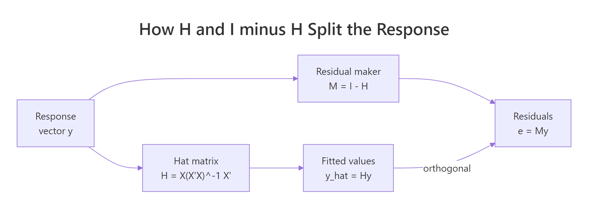
Figure 1: The hat matrix splits y into orthogonal pieces, fitted values Hy and residuals (I − H)y.
Three things to read off this output. First, e_proj matches residuals(model) exactly, the residual maker reproduces R's residual vector. Second, the inner product of fitted values and residuals is essentially zero (orthogonality). Third, $\text{tr}(M) = 29 = 32 - 3$ matches df.residual(model).
Try it: Confirm directly that sum(diag(I - H)) for our 32-by-32 example equals nrow(X) - ncol(X). Reuse M and X.
Click to reveal solution
Explanation: $\text{tr}(I_n - H) = n - \text{tr}(H) = n - p$. The residual subspace has dimension $n - p$, which is what R calls df.residual.
Practice Exercises
These two capstones combine the ideas above. Each exercise uses a fresh prefix (my_) so it does not overwrite the variables from the tutorial.
Exercise 1: Prediction variance from the hat matrix
For the model mpg ~ wt + hp + cyl on mtcars, build the hat matrix from scratch and compute the prediction variance for a new observation with design row $x_* = (1, 3.0, 110, 6)$. The formula is
$$\widehat{\text{Var}}(\hat{y}_) = \hat{\sigma}^2 \left( 1 + x_^\top (X^\top X)^{-1} x_* \right)$$
Save the result to my_pred_var.
Click to reveal solution
Explanation: (X'X)^{-1} falls out of the hat-matrix formula. The inner $x_^\top (X^\top X)^{-1} x_$ measures how far $x_*$ is from the centre of predictor space, far points have larger prediction variance. Adding the $1$ accounts for the irreducible noise in a fresh observation.
Exercise 2: H depends only on the column space, not the columns
Show numerically that adding a redundant column to $X$ (a linear combination of existing columns) leaves the column space, and therefore $H$, unchanged. Build two design matrices: X1 with two columns, and X2 that adds a redundant third column equal to the sum of the first two. Compute both hat matrices (use MASS::ginv() for the rank-deficient $X_2$) and confirm all.equal(H1, H2).
Click to reveal solution
Explanation: $H$ depends only on $\text{col}(X)$, not on which spanning set you pick. Adding a redundant column does not enlarge the column space, so the projection is identical. The pseudo-inverse ginv() is needed because $X_2^\top X_2$ is singular when $X_2$ has redundant columns.
Complete Example: From scratch to lm() diagnostics
Let's walk a single mtcars analysis end-to-end, computing every piece by hand from the hat matrix and confirming each one against R's built-ins. This is the workflow you would use on real data to cross-check lm() output.
Every quantity matches R's built-in functions to machine precision, fitted values, residuals, hat values, and Cook's distance. The Maserati Bora keeps the leverage crown even with qsec added; combined with a moderate residual, it has the highest Cook's distance. Lincoln Continental is high-leverage but well-fit, so its Cook's distance is tiny, exactly the leverage-without-influence pattern called out earlier.
Summary
The hat matrix is the operator that performs the OLS projection. Once you see that, every regression diagnostic looks like a simple geometric measurement.
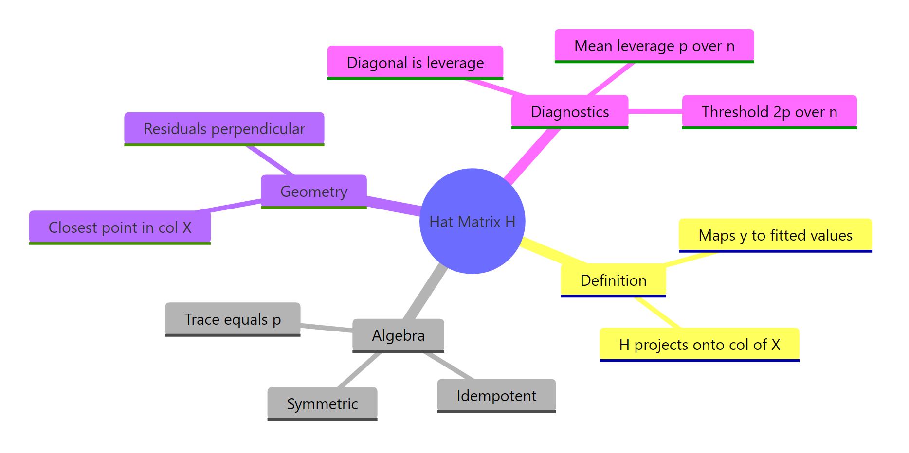
Figure 2: The hat matrix at a glance, definition, algebra, geometry, diagnostics.
| Quantity | Formula | What it measures |
|---|---|---|
| Fitted values | $\hat{y} = Hy$ | Projection of $y$ onto $\text{col}(X)$ |
| Residuals | $e = (I - H)y$ | Component of $y$ orthogonal to $\text{col}(X)$ |
| Leverage | $h_{ii} = (H)_{ii}$ | Self-influence of observation $i$ |
| Mean leverage | $p/n = \text{tr}(H)/n$ | Average self-influence |
| Residual d.f. | $n - p = \text{tr}(I - H)$ | Dimension of the residual subspace |
| Cook's distance | $\frac{h_{ii}}{1 - h_{ii}} \cdot \frac{e_i^2}{p \hat\sigma^2}$ | Combined leverage and residual influence |
Three properties drive everything: $H$ is symmetric, idempotent, and has trace $p$. That is the algebraic signature of an orthogonal projection. Once you accept that signature, residuals, leverage, and degrees of freedom stop being separate formulas and become facets of one geometric picture.
References
- Hastie, T., Tibshirani, R., Friedman, J., The Elements of Statistical Learning, 2nd Edition. Springer (2009). Chapter 3: Linear Methods for Regression. Link
- Wikipedia, Projection matrix. Link
- Strang, G., Introduction to Linear Algebra, 5th Edition. Wellesley-Cambridge Press (2016). Chapter 4: Orthogonality.
- R Core Team,
?hatvaluesand?influence.measures. Link - Faraway, J., Linear Models with R, 2nd Edition. CRC Press (2014). Chapter 6: Diagnostics.
- MIT OpenCourseWare, 18.06 Linear Algebra, Lecture 16: Projection matrices and least squares. Link
- Belsley, D. A., Kuh, E., Welsch, R. E., Regression Diagnostics: Identifying Influential Data and Sources of Collinearity. Wiley (1980).
Continue Learning
- Linear Regression in R, the practical
lm()workflow, coefficient interpretation, andsummary.lm()output. - Outlier Treatment in R, Cook's distance, leverage thresholds, and how to handle influential points.
- Singular Value Decomposition in R, what to do when $X^\top X$ is singular and the standard hat-matrix formula breaks down.