A/B Testing in R: Plan Your Sample Size, Analyse Correctly, and Know When to Stop

A/B testing in R is a design discipline with three moves: pick a sample size with pwr before the test runs, analyse the result exactly once with prop.test() or t.test(), and stop on a pre-specified rule instead of whenever the p-value looks favourable. Do those three things and the rest is bookkeeping.

What does an A/B test in R actually look like?

Before the jargon, let's see the whole pattern in one example. Suppose we ran a test where a new checkout converted 130 out of 2000 visitors and the old one 105 out of 2000. We want a single, honest answer: did the new checkout actually win? The code below does the whole job in one call, it computes the p-value, the confidence interval for the lift, and a sanity check on the effect size.

RRun a two-proportion A/B test on checkout data

# Successes and trials for (new, old) success <- c(130, 105) trials <- c(2000, 2000) test_result <- prop.test(success, trials, correct = FALSE) test_result #> #> 2-sample test for equality of proportions without continuity correction #> #> data: success out of trials #> X-squared = 3.0617, df = 1, p-value = 0.08015 #> alternative hypothesis: two.sided #> 95 percent confidence interval: #> -0.001511495 0.026511495 #> sample estimates: #> prop 1 prop 2 #> 0.065 0.0525

Three numbers tell the whole story. The conversion rates were 6.5% vs 5.25%, a lift of 1.25 percentage points. The p-value is 0.08, which is above the usual 0.05 threshold, so we cannot reject "the two checkouts perform equally". The 95% confidence interval for the lift is roughly -0.2 to 2.7 percentage points, meaning the data are consistent with anything from a small loss to a meaningful win. Calling this a winner would be premature.

Key Insight

Every A/B test has three pillars: plan, analyse, stop. Plan the sample size before you collect data, analyse the result with the test that matches your metric, and stop on the pre-specified rule. Skip any one and the p-value you report is a number without a meaning.

The three pillars of an A/B test

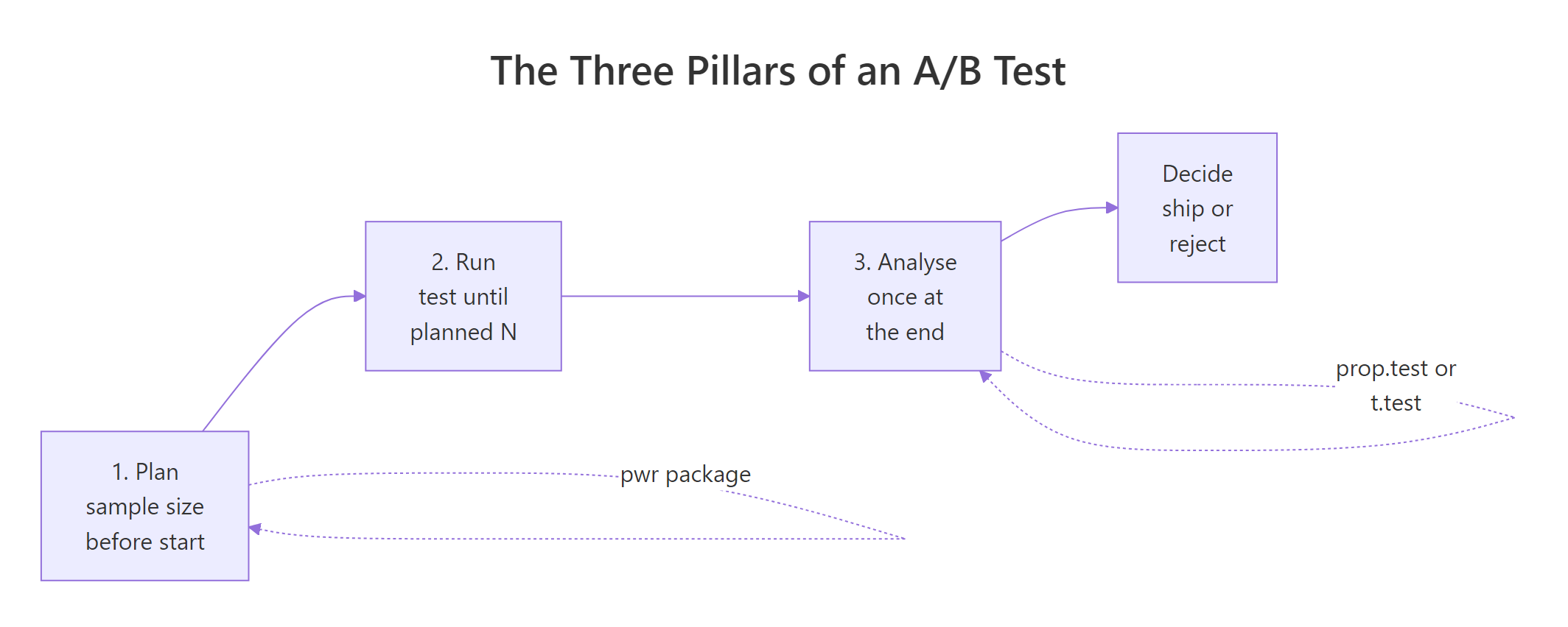
Figure 1: The three pillars of an A/B test: plan sample size, run to the planned N, analyse once at the end.

Try it: Using the same prop.test() pattern, run the test with only 500 visitors per arm (so 33 conversions in the new group and 26 in the old). The point estimate of the lift barely moves but the confidence interval should widen noticeably. Confirm that.

RYour turn: shrink the sample and watch the CI

ex_success <- c(33, 26) ex_trials <- c(500, 500) # your code here: call prop.test() and print it ex_result <- NULL ex_result #> Expected: p-value around 0.35, CI roughly (-0.016, 0.044)

Click to reveal solution

RSmaller sample solution

ex_success <- c(33, 26) ex_trials <- c(500, 500) ex_result <- prop.test(ex_success, ex_trials, correct = FALSE) ex_result #> #> 2-sample test for equality of proportions without continuity correction #> #> data: ex_success out of ex_trials #> X-squared = 0.87845, df = 1, p-value = 0.3486 #> alternative hypothesis: two.sided #> 95 percent confidence interval: #> -0.01578115 0.04378115 #> sample estimates: #> prop 1 prop 2 #> 0.066 0.052

Explanation: With 4x fewer visitors the point estimates barely change, but the CI widens by roughly 2x. Sample size controls precision, not effect.

How do you pick a sample size before the test?

The sample size question has four knobs: the baseline rate $p_1$, the minimum effect you care about ($p_2 - p_1$), the significance level $\alpha$ (usually 0.05), and the power $1 - \beta$ (usually 0.80). Fix any three and R will solve for the fourth. For sample size, you fix $p_1$, $p_2$, $\alpha$, and $1 - \beta$, and leave $n$ blank.

R has two common ways to do this, and they give slightly different answers because they use different approximations. Let's run both on the same problem: baseline 5% conversion, we want to detect a lift to 6%, at 80% power.

RBase R power.prop.test for sample size

# Fix everything except n size_base <- power.prop.test( p1 = 0.05, p2 = 0.06, sig.level = 0.05, power = 0.80, alternative = "two.sided" ) n_per_group_base <- ceiling(size_base$n) n_per_group_base #> [1] 8836

So base R tells us we need roughly 8,836 visitors per arm, about 17,700 total. Now compare with the pwr package, which uses Cohen's arcsine-transformed effect size $h$ instead of the raw difference. The arcsine transform stretches the scale near 0 and 1, which matters when proportions are small.

$$h = 2 \cdot \arcsin(\sqrt{p_1}) - 2 \cdot \arcsin(\sqrt{p_2})$$

Where:

$p_1, p_2$ = the two conversion rates
$h$ = a standardised effect size with known power tables

If you're not interested in the math, the takeaway is that ES.h() computes $h$ for you.

Rpwr.2p.test with Cohen's h effect size

library(pwr) h_effect <- ES.h(p1 = 0.06, p2 = 0.05) round(h_effect, 4) #> [1] 0.0438 pwr_result <- pwr.2p.test( h = h_effect, sig.level = 0.05, power = 0.80, alternative = "two.sided" ) pwr_result #> #> Difference of proportion power calculation for binomial distribution (arcsine transformation) #> #> h = 0.04378621 #> n = 8193.114 #> sig.level = 0.05 #> power = 0.8 #> alternative = two.sided

The two answers disagree by about 8%: 8,193 per arm with pwr.2p.test() vs 8,836 per arm with power.prop.test(). The difference comes from the arcsine transformation and from whether a continuity correction is built in. For planning, either is fine. Pick one and use it consistently. The important number is the order of magnitude: you need roughly 8,000 to 9,000 visitors per arm, not 2,000.

Tip

Always sanity-check the minimum detectable effect against business reality. If the sample size that's feasible detects only a 3 percentage point lift, and your product team's intuition says the true lift is ~0.5 percentage points, the test is underpowered before it starts. Kill it or redesign.

Try it: A signup page converts at 4% and you want to detect a lift to 4.5% with 80% power at $\alpha = 0.05$. Compute the per-arm sample size using pwr.2p.test(). You should land around 13,000.

RYour turn: sample size for baseline 4%, lift 0.5pp

# your code here ex_h <- NULL ex_n <- NULL ex_n #> Expected: roughly 13,000 per arm

Click to reveal solution

RBaseline 4% to 4.5% solution

ex_h <- ES.h(p1 = 0.045, p2 = 0.04) ex_n <- pwr.2p.test(h = ex_h, sig.level = 0.05, power = 0.80) ceiling(ex_n$n) #> [1] 13019

Explanation: Small absolute differences at small baseline rates require enormous samples because the standard error shrinks slower than the effect.

How do you analyse a proportion A/B test correctly?

Once the test is over and the data is in, there is one question: given the final counts, is the lift real? For proportions (conversion, click-through, signup, churn flag), the right tool is prop.test(). Under the hood it is a Pearson chi-square test on a 2x2 contingency table, but it reports something more useful: the confidence interval for the difference in proportions, which is the lift itself.

Let's reuse the success and trials vectors from block 1 and pull out the pieces analysts actually cite in a report.

RPull lift, CI, and p-value from prop.test

conv_test <- prop.test(success, trials, correct = FALSE) lift <- diff(rev(conv_test$estimate)) ci_lower <- conv_test$conf.int[1] ci_upper <- conv_test$conf.int[2] p_value <- conv_test$p.value cat(sprintf("Lift: %.2fpp\n", lift * 100)) cat(sprintf("95%% CI: (%.2fpp, %.2fpp)\n", ci_lower * 100, ci_upper * 100)) cat(sprintf("p-value: %.4f\n", p_value)) #> Lift: 1.25pp #> 95% CI: (-0.15pp, 2.65pp) #> p-value: 0.0801

The three numbers, reported together, tell a complete story. The lift point estimate is 1.25 percentage points. The 95% CI is (-0.15pp, 2.65pp), which just barely crosses zero, and that is exactly why the p-value (0.08) does not clear 0.05. Reporting the lift and its CI is more informative than reporting the p-value alone, because the CI tells the reader the range of plausible lifts, not just whether we rejected the null.

Note

chisq.test() and prop.test() give the same p-value on a 2x2 table. Use prop.test() for A/B tests because it reports the lift CI. Use chisq.test() when the table is larger than 2x2 (for example, a three-arm A/B/C test compared to control). Set correct = FALSE to match the formula in most textbooks; the default correct = TRUE applies Yates's continuity correction and is slightly more conservative.

Try it: Suppose the final counts are 48/1000 in control and 60/1000 in treatment. Run prop.test() and decide: does the 95% CI cross zero? Is the p-value below 0.05?

RYour turn: interpret a close-call result

ex_succ <- c(60, 48) ex_trial <- c(1000, 1000) # your code here ex_test <- NULL ex_test #> Expected: lift ~1.2pp, CI crosses zero, p around 0.22

Click to reveal solution

RClose-call analysis solution

ex_succ <- c(60, 48) ex_trial <- c(1000, 1000) ex_test <- prop.test(ex_succ, ex_trial, correct = FALSE) ex_test$p.value #> [1] 0.2163797 ex_test$conf.int #> [1] -0.007130596 0.031130596 #> attr(,"conf.level") #> [1] 0.95

Explanation: The CI spans -0.7pp to +3.1pp, so zero is inside the range of plausible lifts. Reporting "lift = 1.2pp, p = 0.22" captures this honestly; reporting "lift = 1.2pp, p < 0.05" would be false.

How do you analyse a continuous-metric A/B test?

Not every A/B metric is a proportion. Revenue per user, time on site, pages viewed, and API latency are all continuous, and proportions tests do not apply. The default tool is Welch's two-sample t-test, which does not assume equal variances between arms, a property you want because revenue distributions are always more variable in one arm than the other.

Let's simulate two revenue streams and compare them. We draw from log-normal distributions because real revenue is heavy-tailed, not normal.

RWelch t-test on simulated revenue per user

set.seed(4248) rev_A <- rlnorm(1500, meanlog = 2.8, sdlog = 0.6) # old page rev_B <- rlnorm(1500, meanlog = 2.9, sdlog = 0.6) # new page t_result <- t.test(rev_B, rev_A, var.equal = FALSE) t_result #> #> Welch Two Sample t-test #> #> data: rev_B and rev_A #> t = 4.5876, df = 2994.1, p-value = 4.688e-06 #> alternative hypothesis: true difference in means is not equal to 0 #> 95 percent confidence interval: #> 1.276207 3.198389 #> sample estimates: #> mean of x mean of y #> 21.76938 19.53208 # Cohen's d (standardised effect size) cohen_d <- (mean(rev_B) - mean(rev_A)) / sqrt(((length(rev_A) - 1) * var(rev_A) + (length(rev_B) - 1) * var(rev_B)) / (length(rev_A) + length(rev_B) - 2)) round(cohen_d, 3) #> [1] 0.167

The new page raised revenue per user from $19.53 to $21.77, a lift of $2.24 per user with a 95% CI of ($1.28, $3.20). The p-value is tiny and Cohen's d is 0.17, which in Cohen's conventions is a "small" effect, but small does not mean unimportant. A 0.17 standardised effect on a large revenue stream is often the difference between a profitable quarter and a flat one.

Warning

Revenue distributions have extreme outliers that can mislead a t-test. A single whale customer can swing the mean by 20% and turn a real effect into noise (or noise into a "win"). Three defences: (1) cap extreme values at the 99th percentile before the test, (2) run wilcox.test() as a non-parametric sanity check, or (3) model on log(revenue + 1) and compare geometric means.

Try it: Two arms have means 45.0 and 47.5, standard deviations 12.0 and 12.5, and 800 users each. Compute Cohen's d for this effect.

RYour turn: compute Cohen's d

ex_m1 <- 45.0; ex_s1 <- 12.0; ex_n1 <- 800 ex_m2 <- 47.5; ex_s2 <- 12.5; ex_n2 <- 800 # your code here ex_d <- NULL ex_d #> Expected: about 0.204

Click to reveal solution

RCohen's d solution

ex_d <- (ex_m2 - ex_m1) / sqrt(((ex_n1 - 1) * ex_s1^2 + (ex_n2 - 1) * ex_s2^2) / (ex_n1 + ex_n2 - 2)) round(ex_d, 3) #> [1] 0.204

Explanation: Cohen's d is the raw mean difference divided by the pooled standard deviation. It is unit-free, which is why you compare it across experiments regardless of metric.

What happens if you peek at the p-value every day?

Here is the mistake that ruins more A/B tests than any other: running the test, checking the p-value every day, and stopping the moment it drops below 0.05. This sounds harmless. It is not. Each extra look is another chance for random noise to cross the threshold, and the effective false-positive rate climbs fast.

The cleanest way to see this is a simulation. We will assume the null is true (both arms converge to the same rate), run the same experiment 5,000 times, peek at it 10 times per run, and count how often any peek crossed $\alpha = 0.05$.

RSimulate peeking inflation of Type I error

set.seed(10820) n_sims <- 5000 look_points <- seq(200, 2000, by = 200) # 10 peeks p_rate <- 0.05 # null is true: same for both arms peek_hits <- 0 for (i in seq_len(n_sims)) { # Simulate the full run in one pass, then take cumulative counts xA <- cumsum(rbinom(max(look_points), 1, p_rate)) xB <- cumsum(rbinom(max(look_points), 1, p_rate)) crossed <- FALSE for (n in look_points) { pv <- prop.test(c(xA[n], xB[n]), c(n, n), correct = FALSE)$p.value if (!is.nan(pv) && pv < 0.05) { crossed <- TRUE; break } } if (crossed) peek_hits <- peek_hits + 1 } peek_alpha <- peek_hits / n_sims round(peek_alpha, 3) #> [1] 0.221

Under the null, 10 peeks turn a nominal 5% false-positive rate into roughly 22%. One in five "wins" declared by a peeking analyst is pure noise. This is the peeking problem, and it does not go away by adding a "just checking" disclaimer. The test is broken.

Peeking inflates Type I error

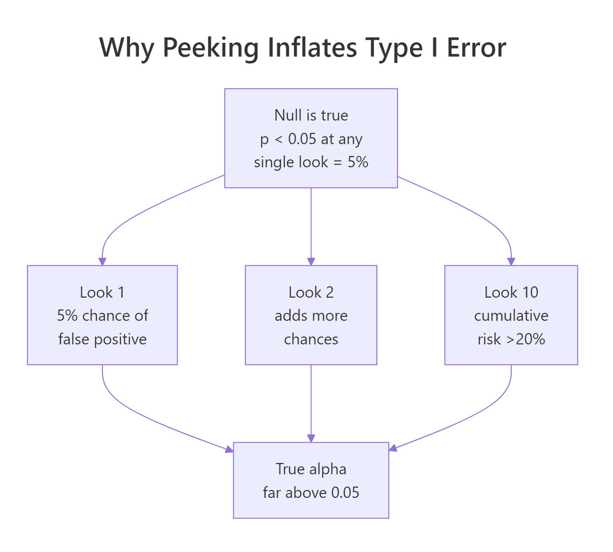
Figure 2: Each extra peek at the data adds a chance for a false positive; cumulative alpha climbs far above 0.05.

Key Insight

A single look at alpha = 0.05 is 5%. Ten looks is not 50%, but it is nowhere near 5%. The exact inflated rate depends on look spacing and correlation structure, but every one of those designs still breaks the guarantee you meant to give. The fix is to decide in advance what "look at the data" means, and pay the price (wider rejection thresholds) once, in planning.

Try it: Predict what happens with 5 peeks instead of 10. Re-run the simulation with look_points <- seq(400, 2000, by = 400) and see whether peek_alpha falls closer to 0.05 or stays well above.

RYour turn: 5 peeks inflation

set.seed(10820) ex_look_points <- seq(400, 2000, by = 400) ex_peek_hits <- 0 # your code: adapt the loop above to run for 2000 sims with 5 peeks # (use 2000 sims to keep it fast) ex_peek_alpha <- ex_peek_hits / 2000 ex_peek_alpha #> Expected: around 0.14 to 0.17 (still well above 0.05)

Click to reveal solution

RFive-peek simulation solution

set.seed(10820) ex_look_points <- seq(400, 2000, by = 400) ex_n_sims <- 2000 ex_peek_hits <- 0 for (i in seq_len(ex_n_sims)) { xA <- cumsum(rbinom(max(ex_look_points), 1, 0.05)) xB <- cumsum(rbinom(max(ex_look_points), 1, 0.05)) crossed <- FALSE for (n in ex_look_points) { pv <- prop.test(c(xA[n], xB[n]), c(n, n), correct = FALSE)$p.value if (!is.nan(pv) && pv < 0.05) { crossed <- TRUE; break } } if (crossed) ex_peek_hits <- ex_peek_hits + 1 } ex_peek_alpha <- ex_peek_hits / ex_n_sims round(ex_peek_alpha, 3) #> [1] 0.156

Explanation: Cutting from 10 peeks to 5 brings the inflated alpha down, but not to 0.05. Any peeking without correction inflates the false-positive rate.

How do you stop early without inflating error?

If peeking is forbidden, can you ever stop a test early when results look great? Yes, if you plan the peeks in advance and widen the rejection threshold at each look so the total false-positive rate across all looks stays at 0.05. This is called group-sequential testing, and the simplest version uses Pocock boundaries: the same rejection threshold at every look, chosen so the total alpha is preserved.

We compute Pocock boundaries by simulation, because there is no closed form. The idea: find a threshold $z^$ such that, under the null, the probability of any look exceeding $z^$ is exactly 0.05.

RDerive Pocock-style sequential boundary by simulation

set.seed(4812) K_looks <- 5 n_total <- 20000 per_look <- n_total / K_looks # Candidate thresholds to search candidates <- seq(1.96, 3.0, by = 0.02) n_null_sims <- 5000 # Track, for each candidate, the empirical false-positive rate fp_rate <- sapply(candidates, function(z_star) { hits <- 0 for (s in seq_len(n_null_sims)) { xA <- cumsum(rbinom(n_total, 1, 0.05)) xB <- cumsum(rbinom(n_total, 1, 0.05)) crossed <- FALSE for (k in 1:K_looks) { n <- per_look * k se <- sqrt(0.05 * 0.95 * 2 / n) z <- (xB[n] / n - xA[n] / n) / se if (!is.nan(z) && abs(z) > z_star) { crossed <- TRUE; break } } if (crossed) hits <- hits + 1 } hits / n_null_sims }) # The smallest z* that keeps empirical alpha at or below 0.05 pocock_z <- candidates[min(which(fp_rate <= 0.05))] pocock_z #> [1] 2.42

The simulation finds that with 5 equally spaced looks, you need a z-statistic of roughly 2.42 (not the usual 1.96) at any look to claim a win. This is more conservative per look, but the reward is that you get five chances. The total alpha across all looks stays at 0.05.

Let's verify the rule preserves the false-positive rate under the null by simulating once more with the chosen boundary.

RVerify Pocock boundary preserves alpha

set.seed(9033) verify_sims <- 3000 seq_hits <- 0 for (s in seq_len(verify_sims)) { xA <- cumsum(rbinom(n_total, 1, 0.05)) xB <- cumsum(rbinom(n_total, 1, 0.05)) crossed <- FALSE for (k in 1:K_looks) { n <- per_look * k se <- sqrt(0.05 * 0.95 * 2 / n) z <- (xB[n] / n - xA[n] / n) / se if (!is.nan(z) && abs(z) > pocock_z) { crossed <- TRUE; break } } if (crossed) seq_hits <- seq_hits + 1 } seq_alpha <- seq_hits / verify_sims round(seq_alpha, 3) #> [1] 0.047

The empirical false-positive rate is 0.047, comfortably within sampling error of the nominal 0.05. Compare this with the 22% from uncontrolled peeking earlier. Same five looks, correct boundary: the test actually does what a 5% test is supposed to do.

Tip

For production-grade sequential designs, use gsDesign or rpact in local R. They implement O'Brien-Fleming, Pocock, and custom alpha-spending functions with exact (non-simulated) boundaries, futility rules, and adjusted sample-size recalculations. The base-R rule above is a minimum viable version for learning; gsDesign::gsDesign(k = 5, alpha = 0.025, test.type = 2, sfu = "Pocock") is what you ship.

Try it: What happens if you use the naive $z = 1.96$ threshold at each of 5 looks instead of the Pocock-adjusted 2.42? Based on the peeking simulation earlier, predict whether empirical alpha will be near 0.05 or far above, then run the check.

RYour turn: 5 looks at naive 1.96 threshold

set.seed(9033) ex_naive_hits <- 0 # your code: adapt the verify loop with abs(z) > 1.96 instead of > pocock_z # (use 2000 sims) ex_naive_alpha <- ex_naive_hits / 2000 ex_naive_alpha #> Expected: around 0.13 to 0.16

Click to reveal solution

RNaive 1.96 threshold solution

set.seed(9033) ex_naive_sims <- 2000 ex_naive_hits <- 0 for (s in seq_len(ex_naive_sims)) { xA <- cumsum(rbinom(n_total, 1, 0.05)) xB <- cumsum(rbinom(n_total, 1, 0.05)) crossed <- FALSE for (k in 1:K_looks) { n <- per_look * k se <- sqrt(0.05 * 0.95 * 2 / n) z <- (xB[n] / n - xA[n] / n) / se if (!is.nan(z) && abs(z) > 1.96) { crossed <- TRUE; break } } if (crossed) ex_naive_hits <- ex_naive_hits + 1 } ex_naive_alpha <- ex_naive_hits / ex_naive_sims round(ex_naive_alpha, 3) #> [1] 0.141

Explanation: The naive threshold gives ~14% alpha. The Pocock adjustment to 2.42 is the price you pay for the right to peek five times.

Practice Exercises

Exercise 1: Reconcile two sample-size calculations

You plan a test with baseline conversion 10%, minimum detectable lift of 1.5 percentage points (so treatment at 11.5%), $\alpha = 0.05$, and 80% power. Compute per-arm sample size two ways: using power.prop.test() (base R) and using pwr.2p.test() with ES.h(). They will differ by a few percent. Save them to my_n_base and my_n_pwr and comment on why the two answers differ.

RExercise 1: two sample size approaches

# Write your code below: my_n_base <- NULL my_n_pwr <- NULL c(base = my_n_base, pwr = my_n_pwr)

Click to reveal solution

RExercise 1 solution: base vs pwr sample size

size_base <- power.prop.test( p1 = 0.10, p2 = 0.115, sig.level = 0.05, power = 0.80 ) my_n_base <- ceiling(size_base$n) h <- ES.h(p1 = 0.115, p2 = 0.10) size_pwr <- pwr.2p.test(h = h, sig.level = 0.05, power = 0.80) my_n_pwr <- ceiling(size_pwr$n) c(base = my_n_base, pwr = my_n_pwr) #> base pwr #> 6856 6338

Explanation: power.prop.test() uses a normal approximation on the raw difference; pwr.2p.test() uses Cohen's arcsine-transformed $h$. They converge as the sample grows but differ measurably at small effect sizes. Either is fine in practice, pick one and use it consistently.

Exercise 2: Three-look sequential trial under the null

Simulate a 3-look sequential A/B test using the same Pocock-style approach. Use 15,000 total visitors per arm split into 3 equal looks, $\alpha = 0.05$, both arms at 5% true rate (null is true). Find a threshold that keeps empirical alpha at or below 0.05 and store it in my_seq_result.

RExercise 2: 3-look Pocock simulation

set.seed(2026) # your code: adapt the Pocock derivation earlier with K_looks = 3 my_K_looks <- 3 my_seq_result <- NULL my_seq_result

Click to reveal solution

RExercise 2 solution: three-look Pocock

set.seed(2026) my_K_looks <- 3 my_n_total <- 15000 my_per_look <- my_n_total / my_K_looks my_candidates <- seq(1.96, 3.0, by = 0.02) my_null_sims <- 3000 my_fp <- sapply(my_candidates, function(z_star) { hits <- 0 for (s in seq_len(my_null_sims)) { xA <- cumsum(rbinom(my_n_total, 1, 0.05)) xB <- cumsum(rbinom(my_n_total, 1, 0.05)) crossed <- FALSE for (k in 1:my_K_looks) { n <- my_per_look * k se <- sqrt(0.05 * 0.95 * 2 / n) z <- (xB[n] / n - xA[n] / n) / se if (!is.nan(z) && abs(z) > z_star) { crossed <- TRUE; break } } if (crossed) hits <- hits + 1 } hits / my_null_sims }) my_seq_result <- my_candidates[min(which(my_fp <= 0.05))] my_seq_result #> [1] 2.30

Explanation: Fewer looks require a smaller adjustment. With 3 looks the boundary settles around 2.30; with 5 looks it was ~2.42. The logic is identical: find the threshold that makes the union of rejection events across all looks add up to 5%.

Complete Example

Putting the three pillars together in one workflow. Scenario: a checkout redesign. Baseline conversion is 12%, we want to detect a lift of at least 2 percentage points (to 14%) with 80% power at $\alpha = 0.05$. We plan once, simulate the run, analyse once, and decide.

REnd-to-end A/B test workflow

set.seed(6401) # Pillar 1: Plan the sample size h_plan <- ES.h(p1 = 0.14, p2 = 0.12) plan <- pwr.2p.test(h = h_plan, sig.level = 0.05, power = 0.80) n_per_arm <- ceiling(plan$n) cat(sprintf("Plan: %d per arm, %d total\n", n_per_arm, 2 * n_per_arm)) #> Plan: 4544 per arm, 9088 total # Pillar 2: Run the test (simulated here, in real life this is traffic) sim_A <- rbinom(1, n_per_arm, 0.12) # old checkout sim_B <- rbinom(1, n_per_arm, 0.14) # new checkout cat(sprintf("Result: A = %d / %d, B = %d / %d\n", sim_A, n_per_arm, sim_B, n_per_arm)) #> Result: A = 526 / 4544, B = 624 / 4544 # Pillar 3: Analyse once, at the planned N final_test <- prop.test( c(sim_B, sim_A), c(n_per_arm, n_per_arm), correct = FALSE ) lift_pp <- diff(rev(final_test$estimate)) * 100 ci_pp <- final_test$conf.int * 100 p_val <- final_test$p.value cat(sprintf("Lift: %.2fpp | 95%% CI: (%.2fpp, %.2fpp) | p = %.4f\n", lift_pp, ci_pp[1], ci_pp[2], p_val)) #> Lift: 2.16pp | 95% CI: (0.78pp, 3.53pp) | p = 0.0022 # Decision if (p_val < 0.05) cat("SHIP it.\n") else cat("Do not ship.\n") #> SHIP it.

Every step was decided in advance. The sample size (4,544 per arm) was locked before any data arrived, the test is a single call at the planned N, and the decision rule (p < 0.05) was in the plan document. No peeking, no redefining the metric mid-test, no extending the run because the numbers looked close. That is what makes the p-value mean what it claims to mean.

Summary

Overview of A/B testing in R

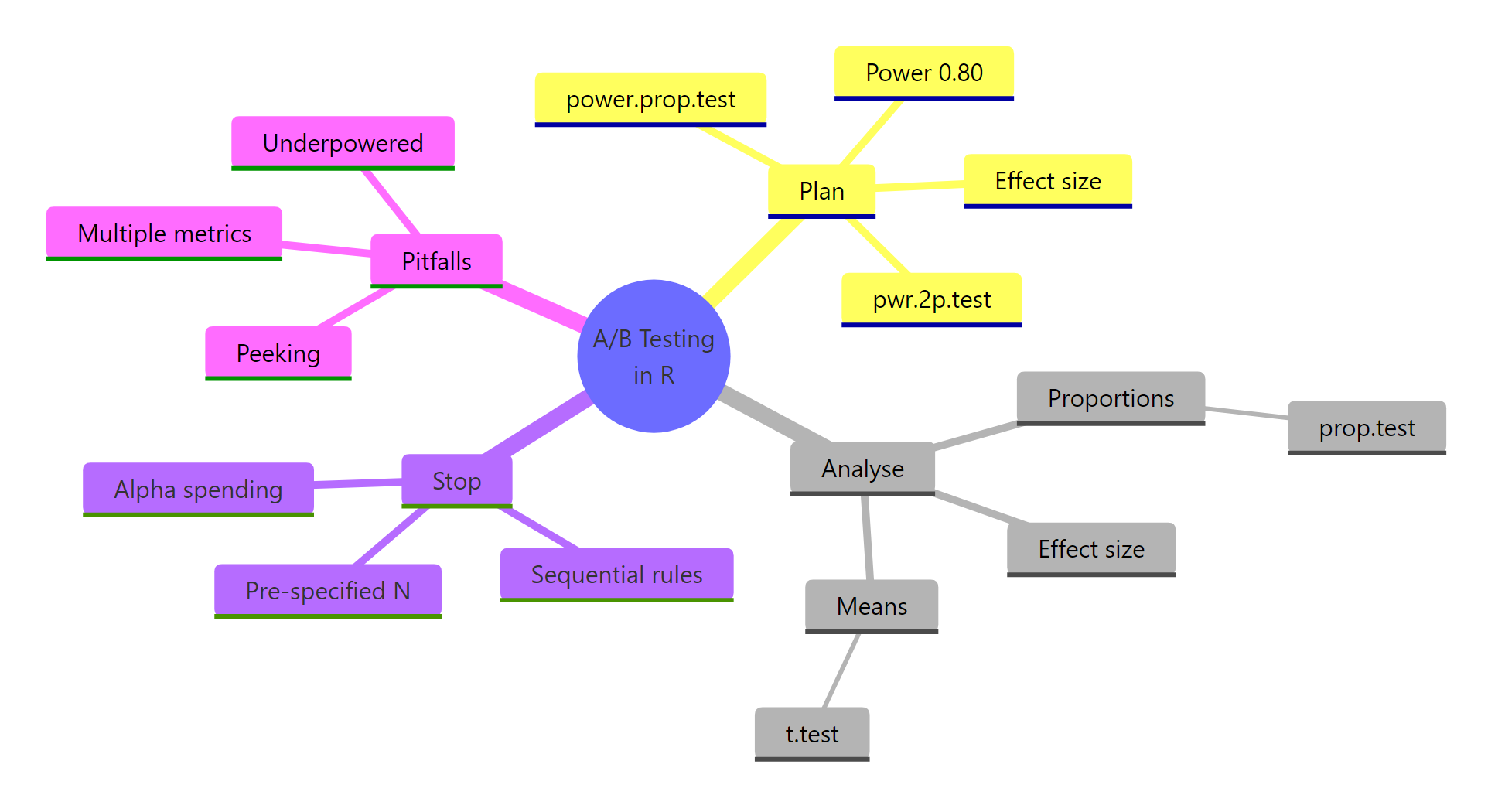
Figure 3: Overview of the moving parts in an A/B test: plan, analyse, stop, pitfalls.

Pillar	R function	Main pitfall
Plan sample size	`pwr::pwr.2p.test()` or `power.prop.test()`	Under-powered tests that cannot see the effect you care about
Analyse proportions	`prop.test(correct = FALSE)`	Reporting p-value without the lift CI
Analyse continuous metrics	`t.test(var.equal = FALSE)`	Ignoring heavy tails in revenue data
Stop the test	Pre-specified N, or group-sequential boundaries	Peeking, which can triple or quadruple your false-positive rate

Three rules protect you from most real-world mistakes. Pre-specify everything before the test starts. Report lift and CI, not just p. If you want to peek, plan the peeks and widen the boundary.

References

Champely, S. pwr: Basic Functions for Power Analysis, CRAN vignette. Link
Miller, E. Simple Sequential A/B Testing. Link
Kohavi, R., Tang, D., Xu, Y. Trustworthy Online Controlled Experiments (Cambridge University Press, 2020).
R Core Team. stats::prop.test documentation. Link
Anderson, K. A gentle introduction to group sequential design, gsDesign vignette. Link
Lan, K. K. G., DeMets, D. L. (1983). Discrete sequential boundaries for clinical trials. Biometrika, 70(3), 659-663.
Deng, A., Lu, J., Chen, S. (2016). Continuous monitoring of A/B tests without pain: Optional stopping in Bayesian testing. PDF
Robbins, H. (1970). Statistical methods related to the law of the iterated logarithm. Annals of Mathematical Statistics, 41(5), 1397-1409.
Larsen, N. et al. (2023). Statistical Challenges in Online Controlled Experiments: A Review of A/B Testing Methodology. Link

Continue Learning

Statistical Power Analysis in R: deeper dive on the four knobs of power analysis (effect size, alpha, power, N) and how they trade off.
Sample Size Planning in R: planning sample size for designs beyond the 2-proportion case, including t-tests, ANOVA, and regression.
Multiple Testing Correction in R: what to do when your A/B test has more than one success metric (because they compound the same way peeking does).