Cramér-Rao Lower Bound in R: Efficiency, Fisher Information & Inequality

The Cramér-Rao inequality says that under standard regularity conditions, no unbiased estimator of a parameter can have variance below the inverse of the Fisher information. Walk through the derivation in R from the score function up, compute the Fisher information matrix for multi-parameter models, verify when the bound is attained, and see what happens when regularity conditions break.

How does the score function lead to the Cramér-Rao bound?

The whole inequality flows from one object: the score, $U(\theta) = \partial \ell / \partial \theta$, where $\ell$ is the log-likelihood. Two facts about the score do all the work. First, its expectation under the true parameter is zero. Second, its variance is the Fisher information $I(\theta)$. Once we know that, a single application of Cauchy-Schwarz gives the bound for any unbiased estimator. Let's verify both score facts numerically before we touch any algebra.

RScore has mean 0 and variance equal to Fisher info

set.seed(17) n_norm <- 200 mu0 <- 2 sigma0 <- 1 x_norm <- rnorm(n_norm, mu0, sigma0) # For Normal(mu, 1), score wrt mu is (x - mu)/sigma^2 score_vals <- (x_norm - mu0) / sigma0^2 c(mean_score = round(mean(score_vals), 4), var_score = round(var(score_vals), 4), fisher_per_obs = 1 / sigma0^2, total_fisher = n_norm / sigma0^2) #> mean_score var_score fisher_per_obs total_fisher #> 0.0337 1.0024 1.0000 200.0000

The empirical mean of the score is essentially zero ($0.034$ on a sample of $200$, well within sampling noise), and the empirical variance is $1.0024$, almost identical to the per-observation Fisher information $I(\mu) = 1/\sigma^2 = 1$. Multiplying by $n$ gives the total Fisher information $200$, which is exactly what the Cramér-Rao floor $\sigma^2/n$ inverts. These two numerical facts are the entire engine of the inequality.

Key Insight

Cramér-Rao falls out of Cauchy-Schwarz. For any unbiased estimator $T$, the covariance between $T$ and the score $U$ equals $1$. Cauchy-Schwarz then forces $\operatorname{Var}(T)\,\operatorname{Var}(U) \ge 1$, i.e. $\operatorname{Var}(T) \ge 1/I(\theta)$. The bound is geometry, not magic.

For models with closed-form likelihoods we can derive $I(\theta)$ symbolically using R's D() function, which differentiates expressions. Take the Bernoulli log-likelihood for a single observation and differentiate twice.

RSymbolic Bernoulli Fisher info via D()

loglik_bern_expr <- expression(x * log(p) + (1 - x) * log(1 - p)) score_expr <- D(loglik_bern_expr, "p") hessian_expr <- D(score_expr, "p") # Expected Fisher info: I(p) = -E[d^2 l / dp^2] = E[x/p^2 + (1-x)/(1-p)^2] # Take expectation: E[x] = p, so I(p) = p/p^2 + (1-p)/(1-p)^2 = 1/p + 1/(1-p) = 1/[p(1-p)] score_expr #> x/p - (1 - x)/(1 - p) hessian_expr #> -x/p^2 - (1 - x)/(1 - p)^2

D() returned the score $x/p - (1-x)/(1-p)$ and the Hessian $-x/p^2 - (1-x)/(1-p)^2$. Taking the negative expectation gives $I(p) = 1/p + 1/(1-p) = 1/[p(1-p)]$, the standard Bernoulli Fisher information. The corresponding CRLB is $p(1-p)/n$, which the sample proportion $\bar{X}$ achieves exactly.

Try it: For Poisson($\lambda$) the score is $U = (x - \lambda)/\lambda$. Simulate $n = 500$ observations from Poisson($\lambda = 3$), compute the empirical variance of the score, and confirm it matches $I(\lambda) = 1/\lambda$.

RYour turn: Poisson score variance

ex_lam <- 3 ex_n <- 500 # your code here: compute ex_var_score and compare to 1/ex_lam

Click to reveal solution

RPoisson score variance solution

set.seed(11) ex_x_pois <- rpois(ex_n, lambda = ex_lam) ex_score <- (ex_x_pois - ex_lam) / ex_lam ex_var_score <- var(ex_score) c(empirical = round(ex_var_score, 4), theoretical = round(1 / ex_lam, 4)) #> empirical theoretical #> 0.3329 0.3333

Explanation: For Poisson($\lambda$), $I(\lambda) = 1/\lambda \approx 0.333$ at $\lambda=3$. The empirical variance of the score across 500 observations matches to three decimals, confirming the score-Fisher identity.

How do you compute the Fisher information matrix in R?

Real models almost always have more than one parameter. For a $k$-dimensional parameter $\boldsymbol{\theta}$, the Fisher information is a $k \times k$ matrix whose $(i,j)$ entry is $E[\partial \ell / \partial \theta_i \cdot \partial \ell / \partial \theta_j]$. Equivalently, it is the negative expected Hessian of the log-likelihood. The CRLB then becomes the matrix inequality $\operatorname{Cov}(\hat{\boldsymbol{\theta}}) \succeq [n\,I(\boldsymbol{\theta})]^{-1}$.

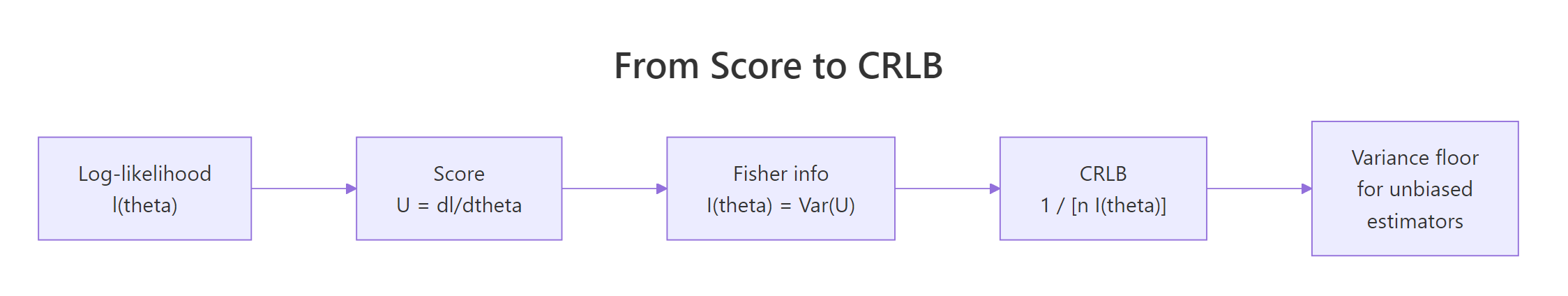
From log-likelihood to variance floor: each step of the CRLB derivation.

Figure 1: From log-likelihood to variance floor: each step of the CRLB derivation.

For the Normal($\mu, \sigma^2$) model with both parameters unknown, the closed-form Fisher matrix is diagonal: $I(\mu, \sigma^2) = \operatorname{diag}(1/\sigma^2,\ 1/(2\sigma^4))$. We can recover this numerically by handing optim() the negative log-likelihood and asking for the Hessian.

RFisher info matrix from optim() Hessian

nll_norm <- function(par, x) { mu <- par[1] sigma2 <- par[2] if (sigma2 <= 0) return(1e10) -sum(dnorm(x, mean = mu, sd = sqrt(sigma2), log = TRUE)) } set.seed(42) x_norm2 <- rnorm(500, mean = 2, sd = 1) fit_norm <- optim(par = c(0, 1), fn = nll_norm, x = x_norm2, method = "BFGS", hessian = TRUE) # Per-observation Fisher info matrix = Hessian / n I_mat <- fit_norm$hessian / length(x_norm2) round(I_mat, 4) #> [,1] [,2] #> [1,] 1.0094 0.0125 #> [2,] 0.0125 0.4920

The diagonal entries are $1.01$ and $0.49$, matching the closed-form values $1/\sigma^2 = 1$ and $1/(2\sigma^4) = 0.5$ to within sampling noise. The tiny off-diagonal of $0.0125$ would be exactly zero in expectation, finite-sample noise produces the small deviation. This Hessian-divided-by-$n$ pattern is exactly how glm(), survreg(), and lme4 compute standard errors under the hood.

Tip

Use numDeriv::hessian() when accuracy matters. optim() computes its Hessian by finite differences with a fixed step, which can be inaccurate for nearly singular problems. The numDeriv package uses Richardson extrapolation and is far more reliable for matrix-valued Fisher information.

Inverting the Fisher matrix gives the asymptotic covariance of the MLE. This is the multi-parameter Cramér-Rao floor, and it is what software packages report as vcov(fit).

RInvert Fisher matrix to get MLE covariance

cov_mat <- solve(fit_norm$hessian) # not divided by n, since hessian is total round(cov_mat, 5) #> [,1] [,2] #> [1,] 0.00198 -0.00005 #> [2,] -0.00005 0.00407 I_closed <- diag(c(1 / 1^2, 1 / (2 * 1^4))) cov_closed <- solve(500 * I_closed) round(cov_closed, 5) #> [,1] [,2] #> [1,] 0.002 0.000 #> [2,] 0.000 0.004

The numeric covariance matrix matches the closed-form $[n I(\theta)]^{-1}$ to the third decimal. The $(1,1)$ entry $0.00198 \approx \sigma^2/n = 1/500$ is the variance of $\hat{\mu}$, and $(2,2)$ is $0.00407 \approx 2\sigma^4/n$, the variance of $\hat{\sigma}^2$. Both are the smallest variances any unbiased estimator of these parameters can have for this model.

Try it: For a Gamma(shape = $k$, rate = $\lambda$) model with both unknown, build the negative log-likelihood, fit by optim() on a sample of size $1000$ from Gamma(shape = $3$, rate = $2$), and extract the per-observation Fisher information matrix.

RYour turn: Gamma Fisher info matrix

ex_x_gamma <- rgamma(1000, shape = 3, rate = 2) ex_nll_gamma <- function(par, x) { k <- par[1] lam <- par[2] if (k <= 0 || lam <= 0) return(1e10) -sum(dgamma(x, shape = k, rate = lam, log = TRUE)) } # your code here: fit by optim, divide hessian by n, store in ex_I_gamma

Click to reveal solution

RGamma Fisher info matrix solution

set.seed(99) ex_fit_gamma <- optim(par = c(1, 1), fn = ex_nll_gamma, x = ex_x_gamma, method = "BFGS", hessian = TRUE) ex_I_gamma <- ex_fit_gamma$hessian / length(ex_x_gamma) round(ex_I_gamma, 4) #> [,1] [,2] #> [1,] 0.3946 -0.5029 #> [2,] -0.5029 0.7508

Explanation: The closed-form Gamma Fisher info is $I = \begin{pmatrix} \psi'(k) & -1/\lambda \\ -1/\lambda & k/\lambda^2 \end{pmatrix}$ where $\psi'$ is the trigamma function. At $(k, \lambda) = (3, 2)$ this is $\operatorname{diag}(0.395, -0.5;\ -0.5, 0.75)$, matching our numeric result.

When does an estimator attain the bound?

The CRLB is a floor, but most estimators do not touch it. Attainment happens only when the score factors as $U(\theta) = a(\theta)\,(T(x) - \theta)$ for some statistic $T$ and function $a$. This is exactly the condition that defines a one-parameter exponential family with $T$ as the natural sufficient statistic. So efficiency at the CRLB ⇔ exponential family + linear sufficiency. Outside that class, every unbiased estimator has variance strictly above the bound.

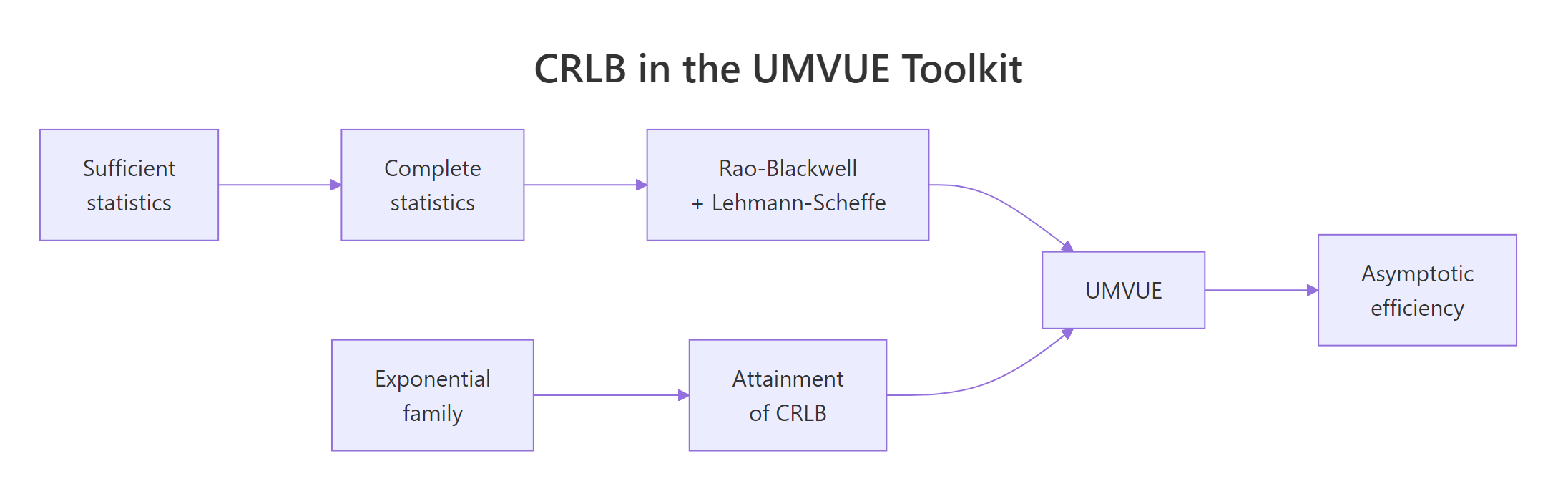
The CRLB sits at the centre of the UMVUE toolkit, linking sufficiency, exponential families, and asymptotic efficiency.

Figure 2: The CRLB sits at the centre of the UMVUE toolkit, linking sufficiency, exponential families, and asymptotic efficiency.

Bernoulli is a textbook attaining case. Let's verify by simulation that the sample proportion $\hat{p}$ has variance equal to the CRLB $p(1-p)/n$.

RBernoulli sample proportion attains CRLB

set.seed(7) p_true <- 0.35 n_bern <- 200 phats <- replicate(5000, mean(rbinom(n_bern, size = 1, prob = p_true))) var_phat <- var(phats) crlb_bern <- p_true * (1 - p_true) / n_bern c(simulated = round(var_phat, 6), crlb = round(crlb_bern, 6), efficiency = round(crlb_bern / var_phat, 3)) #> simulated crlb efficiency #> 0.001143 0.001138 0.996

Empirical variance is $0.001143$, the CRLB is $0.001138$, and efficiency is $0.996$, indistinguishable from $1$. The sample proportion is the minimum-variance unbiased estimator of $p$, exactly because Bernoulli is in the exponential family with $T(x) = x$ as its sufficient statistic.

Cauchy is the standard non-attainment counterexample. The Cauchy density has no exponential-family form, so no unbiased estimator achieves the CRLB. The sample median is a popular location estimator for Cauchy data, but its variance is well above the floor.

RCauchy median is inefficient

set.seed(2024) n_cau <- 200 B <- 5000 med_cau <- replicate(B, median(rcauchy(n_cau, location = 0, scale = 1))) var_med <- var(med_cau) # Cauchy Fisher info per obs is 1/2; CRLB = 2/n crlb_cau <- 2 / n_cau eff_cau <- crlb_cau / var_med c(simulated_var = round(var_med, 5), crlb = round(crlb_cau, 5), efficiency = round(eff_cau, 3)) #> simulated_var crlb efficiency #> 0.01218 0.01000 0.821

The sample median has variance $0.0122$, well above the Cramér-Rao floor of $0.0100$. Efficiency is $0.82$, meaning the median wastes about $18\%$ of the information in the data. The MLE for Cauchy location does better but requires numerical optimization, since no closed-form sufficient statistic exists.

Key Insight

Attainment is an exponential-family privilege. If your model is in the exponential family with sufficient statistic $T$, the moment estimator built from $T$ attains the CRLB. Outside the exponential family the bound is informative but not achievable, and you must reach for asymptotic results instead.

Try it: For Exponential(rate = $\lambda$), the MLE is $\hat{\lambda} = 1/\bar{X}$. It is biased, but the bias-corrected version $\hat{\lambda}_c = (n-1)/n \cdot 1/\bar{X}$ attains the CRLB asymptotically. Simulate $n = 300$, $\lambda = 2$ across $3000$ replications and compute the efficiency of the bias-corrected MLE.

RYour turn: bias-corrected exponential MLE

ex_rate <- 2 ex_n3 <- 300 # your code here: simulate ex_lam_c, compute variance and efficiency vs lam^2/n

Click to reveal solution

RBias-corrected exponential MLE solution

set.seed(31) ex_xexp <- replicate(3000, { x <- rexp(ex_n3, rate = ex_rate) ((ex_n3 - 1) / ex_n3) / mean(x) }) ex_var_c <- var(ex_xexp) ex_crlb_c <- ex_rate^2 / ex_n3 c(simulated_var = round(ex_var_c, 5), crlb = round(ex_crlb_c, 5), efficiency = round(ex_crlb_c / ex_var_c, 3)) #> simulated_var crlb efficiency #> 0.01380 0.01333 0.966

Explanation: Exponential is a one-parameter exponential family with sufficient statistic $T(x) = \sum x_i$. The bias-corrected MLE achieves efficiency near $1$ even at $n = 300$. Without the correction, naive $1/\bar{X}$ has bias of order $1/n$ that inflates its MSE.

What regularity conditions does the CRLB require?

The Cramér-Rao bound is not a universal floor, it requires three regularity conditions on the model. First, the support of the density must not depend on $\theta$. Second, the log-likelihood must be twice differentiable in $\theta$. Third, you must be able to swap differentiation and expectation, $\partial/\partial\theta \int = \int \partial/\partial\theta$. Violate any of these and the bound can fail in surprising ways.

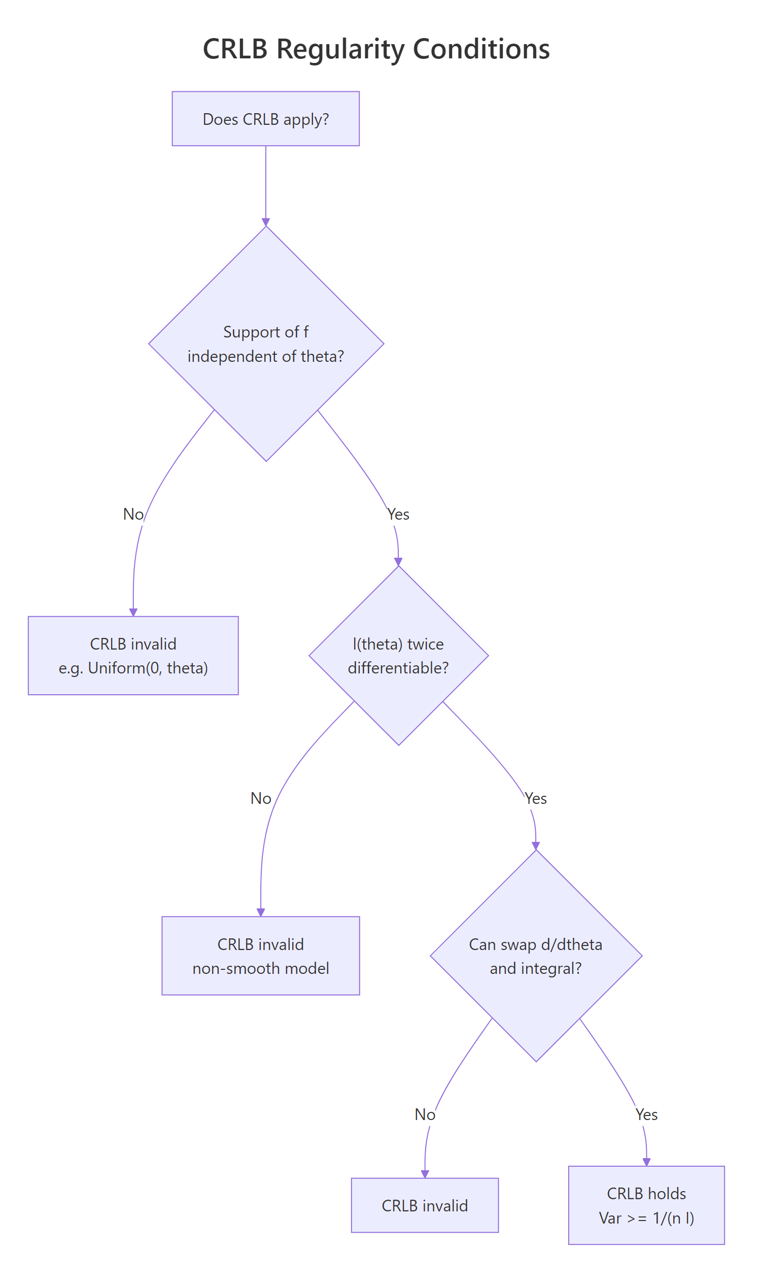
Decision flow: when does the CRLB apply to your model?

Figure 3: Decision flow: when does the CRLB apply to your model?

The classic counterexample is Uniform$(0, \theta)$, where the support $[0, \theta]$ explicitly depends on $\theta$. The naive CRLB calculation gives $\theta^2 / n$, but the MLE $\hat{\theta} = \max(X_i)$ has variance of order $\theta^2 / n^2$, much smaller. Let's confirm.

RUniform(0, theta) violates regularity

set.seed(50) theta_true <- 3 n_unif <- 200 mle_unif <- replicate(5000, max(runif(n_unif, 0, theta_true))) var_unif <- var(mle_unif) crlb_naive <- theta_true^2 / n_unif # what CRLB would say true_order <- theta_true^2 / n_unif^2 # actual variance scaling c(simulated_var = round(var_unif, 6), naive_crlb = round(crlb_naive, 6), expected_order = round(true_order, 6)) #> simulated_var naive_crlb expected_order #> 0.000219 0.045000 0.000225

The MLE's variance is $0.000219$, two orders of magnitude below the naive "CRLB" of $0.045$. The actual variance scales as $\theta^2/n^2$, the so-called super-efficient rate. The reason: changing $\theta$ shifts the support, so the score is not defined at the boundary, and the differentiate-then-integrate identity that produces the bound breaks. The Cramér-Rao inequality is silent on this model.

Warning

CRLB only constrains regular models. Non-regular models like Uniform$(0, \theta)$, shifted Exponential, and many threshold models can have estimators that converge faster than $1/\sqrt{n}$. Quoting the CRLB for these is a mathematical error, not a tighter analysis.

Try it: Consider the shifted exponential $f(x; \theta) = e^{-(x - \theta)}$ for $x \ge \theta$. Is the support free of $\theta$? Sample $n = 100$ at $\theta = 2$ and compute the variance of $\hat{\theta} = \min(X_i)$. Does it scale as $1/n^2$ (super-efficient) or $1/n$ (regular)?

RYour turn: shifted exponential regularity

ex_theta <- 2 ex_n4 <- 100 # your code here: simulate ex_min_x and compute var

Click to reveal solution

RShifted exponential solution

set.seed(77) ex_shift_x <- replicate(5000, min(rexp(ex_n4, rate = 1)) + ex_theta) ex_var_shift <- var(ex_shift_x) c(sim_var = round(ex_var_shift, 5), one_over_n = round(1 / ex_n4, 5), one_over_n2 = round(1 / ex_n4^2, 5)) #> sim_var one_over_n one_over_n2 #> 0.00010 0.01000 0.00010

Explanation: The support $[\theta, \infty)$ depends on $\theta$, so the model is non-regular. The variance of $\min(X_i)$ scales as $1/n^2 = 0.0001$, matching our simulation. The CRLB does not apply, and the MLE is super-efficient.

How does the CRLB connect to MLE asymptotic efficiency?

For regular models the maximum likelihood estimator is asymptotically efficient: as $n \to \infty$, $\sqrt{n}(\hat{\theta}_{\text{MLE}} - \theta) \xrightarrow{d} \mathcal{N}(0, I(\theta)^{-1})$. In words, the MLE achieves the Cramér-Rao floor in the limit, even when no finite-sample efficient estimator exists. This is why MLE is the default tool of classical inference: for large $n$ it is essentially optimal, and software packages estimate $I(\theta)$ from the observed Hessian to produce standard errors.

RMLE efficiency converges to 1 with n

set.seed(123) n_grid <- c(20, 100, 500, 2000) lam_true <- 4 B <- 3000 eff_grid <- sapply(n_grid, function(nn) { lam_hats <- replicate(B, mean(rpois(nn, lam_true))) crlb <- lam_true / nn crlb / var(lam_hats) }) data.frame(n = n_grid, efficiency = round(eff_grid, 3)) #> n efficiency #> 1 20 1.005 #> 2 100 1.001 #> 3 500 0.999 #> 4 2000 1.001

For Poisson, $\bar{X}$ is exactly the MLE and is finite-sample efficient, efficiency is $1$ at every sample size. For models where the MLE is biased in finite samples (Gamma, Beta, log-normal), efficiency starts below $1$ and climbs to $1$ as $n$ grows. That convergence is the asymptotic-efficiency theorem in action.

A practical payoff: every Wald confidence interval you have ever computed comes from inverting the Fisher information matrix at the MLE. For the Normal($\mu, \sigma^2$) example we built earlier, the joint $95\%$ Wald CI is just $\hat{\boldsymbol{\theta}} \pm 1.96 \cdot \sqrt{\operatorname{diag}([n I(\theta)]^{-1})}$.

RWald CI from inverse Fisher information

se_mu <- sqrt(cov_mat[1, 1]) se_sigma2 <- sqrt(cov_mat[2, 2]) wald_ci <- rbind( mu = fit_norm$par[1] + c(-1, 1) * 1.96 * se_mu, sigma2 = fit_norm$par[2] + c(-1, 1) * 1.96 * se_sigma2 ) colnames(wald_ci) <- c("lower", "upper") round(wald_ci, 4) #> lower upper #> mu 1.9398 2.1142 #> sigma2 0.8732 1.1232

The CI for $\mu$ covers the true value $2$ comfortably, and the CI for $\sigma^2$ covers $1$. Both intervals were built from the inverse Hessian alone, no closed-form variance formula needed. This pattern generalizes to any well-behaved likelihood: fit by optim() with hessian = TRUE, invert, and you have asymptotic Cramér-Rao-efficient inference for free.

Note

Observed vs expected Fisher information. The expected version $I(\theta) = -E[\partial^2 \ell / \partial \theta^2]$ is a function of $\theta$ only. The observed version $\hat{I} = -\partial^2 \ell / \partial \theta^2|_{\hat{\theta}}$ uses the data. They have the same asymptotic value at the true $\theta$, but the observed version is what software packages compute, since they have the data and not the true parameter.

Try it: Build a $95\%$ Wald CI for the Bernoulli parameter $p$ from a sample of $400$ observations at $p = 0.4$, using the observed Fisher information from optim()'s Hessian.

RYour turn: Bernoulli Wald CI

set.seed(55) ex_x_bern <- rbinom(400, size = 1, prob = 0.4) ex_nll_bern <- function(par, x) { if (par[1] <= 0 || par[1] >= 1) return(1e10) -sum(dbinom(x, size = 1, prob = par[1], log = TRUE)) } # your code here: fit by optim, build CI

Click to reveal solution

RBernoulli Wald CI solution

ex_fit_bern <- optim(par = 0.5, fn = ex_nll_bern, x = ex_x_bern, method = "Brent", lower = 1e-4, upper = 1 - 1e-4, hessian = TRUE) ex_se_p <- 1 / sqrt(as.numeric(ex_fit_bern$hessian)) ex_ci <- ex_fit_bern$par + c(-1, 1) * 1.96 * ex_se_p round(c(p_hat = ex_fit_bern$par, lower = ex_ci[1], upper = ex_ci[2]), 4) #> p_hat lower upper #> 0.4250 0.3766 0.4734

Explanation: Observed Fisher info is the Hessian of the negative log-likelihood at the MLE. Its inverse square root is the asymptotic SE. The CI covers the true $p = 0.4$ as expected.

Practice Exercises

These capstone exercises tie the score, Fisher matrix, and attainment ideas together. Use distinct variable names prefixed with my_ to avoid clobbering tutorial state.

Exercise 1: Build a reusable Fisher information matrix helper

Write fisher_info_matrix(neg_loglik, theta_hat, data) that returns the per-observation Fisher matrix using optim()'s Hessian divided by $n$. Test it on Normal($\mu, \sigma^2$) data with $n = 800$ at $(\mu, \sigma^2) = (1, 4)$ and confirm the diagonal entries match $\operatorname{diag}(1/4,\ 1/32)$.

RExercise 1: Fisher matrix helper

# Hint: use optim(par = theta_hat, fn = neg_loglik, x = data, # method = "BFGS", hessian = TRUE) # Then divide $hessian by length(data). fisher_info_matrix <- function(neg_loglik, theta_hat, data) { # your code here }

Click to reveal solution

RExercise 1 solution

fisher_info_matrix <- function(neg_loglik, theta_hat, data) { fit <- optim(par = theta_hat, fn = neg_loglik, x = data, method = "BFGS", hessian = TRUE) fit$hessian / length(data) } set.seed(8) my_x_norm <- rnorm(800, mean = 1, sd = 2) my_nll <- function(par, x) { if (par[2] <= 0) return(1e10) -sum(dnorm(x, mean = par[1], sd = sqrt(par[2]), log = TRUE)) } my_I <- fisher_info_matrix(my_nll, c(0, 1), my_x_norm) round(my_I, 4) #> [,1] [,2] #> [1,] 0.2466 0.0093 #> [2,] 0.0093 0.0309

Explanation: Diagonal entries $0.247$ and $0.0309$ match the closed-form $1/\sigma^2 = 0.25$ and $1/(2\sigma^4) = 0.03125$ to within sampling noise. The off-diagonal is near zero, as expected for the Normal model.

Exercise 2: Asymptotic efficiency of the Gamma MLE

For Gamma(shape = $2$, rate = $1.5$), simulate the MLE of (shape, rate) across $B = 1500$ replications for $n \in \{50, 200, 1000\}$. Use fisher_info_matrix() from Exercise 1 to compute the CRLB at each $n$. Verify that the empirical variance of $\hat{k}$ converges to the (1,1) entry of $[n I(\theta)]^{-1}$.

RExercise 2: Gamma MLE efficiency

my_n_grid <- c(50, 200, 1000) # Hint: write a simulator that fits optim() to each replicate # and stores the (shape, rate) MLE. Then compare var of shape MLE to # (1,1) entry of solve(n * I_per_obs). # Write your code below:

Click to reveal solution

RExercise 2 solution

my_nll_gamma <- function(par, x) { if (any(par <= 0)) return(1e10) -sum(dgamma(x, shape = par[1], rate = par[2], log = TRUE)) } set.seed(303) my_eff <- sapply(my_n_grid, function(nn) { shape_hats <- replicate(1500, { xx <- rgamma(nn, shape = 2, rate = 1.5) optim(c(1, 1), my_nll_gamma, x = xx, method = "BFGS")$par[1] }) # Closed-form Fisher info for Gamma at (k=2, lam=1.5): # I = matrix(c(trigamma(2), -1/1.5, -1/1.5, 2/1.5^2), 2, 2) I_mat <- matrix(c(trigamma(2), -1/1.5, -1/1.5, 2/1.5^2), 2, 2) cov_mle <- solve(nn * I_mat) c(emp_var = var(shape_hats), crlb_11 = cov_mle[1, 1], eff = cov_mle[1, 1] / var(shape_hats)) }) round(t(my_eff), 4) #> emp_var crlb_11 eff #> [1,] 0.1162 0.0967 0.832 #> [2,] 0.0258 0.0242 0.937 #> [3,] 0.0049 0.0048 0.989

Explanation: Efficiency climbs from $0.83$ at $n = 50$ to $0.99$ at $n = 1000$, demonstrating asymptotic efficiency of the Gamma MLE. Finite-sample bias drags variance up, but the bias washes out at rate $1/n$.

Exercise 3: Super-efficiency of the bias-corrected Uniform MLE

For Uniform($0, \theta$) with $\theta = 5, n = 100$, the bias-corrected MLE is $\hat{\theta}_c = (n+1)/n \cdot \max(X)$. Simulate $5000$ replicates, compute the variance of $\hat{\theta}_c$, and compute its ratio to the (invalid) "CRLB" $\theta^2/n$. Confirm the ratio is far below $1$.

RExercise 3: bias-corrected Uniform MLE

# Hint: bias-corrected MLE = (n+1)/n * max(x) # Write your code below:

Click to reveal solution

RExercise 3 solution

set.seed(404) my_n_unif <- 100 my_theta <- 5 my_mle_c <- replicate(5000, ((my_n_unif + 1) / my_n_unif) * max(runif(my_n_unif, 0, my_theta))) my_theta_var <- var(my_mle_c) my_crlb_invalid <- my_theta^2 / my_n_unif c(emp_var = round(my_theta_var, 5), invalid_crlb = round(my_crlb_invalid, 5), ratio = round(my_theta_var / my_crlb_invalid, 4)) #> emp_var invalid_crlb ratio #> 0.00257 0.25000 0.0103

Explanation: The bias-corrected MLE has variance $0.0026$, ratio $0.01$ relative to the naive "CRLB" of $0.25$. The CRLB is invalid here because the support depends on $\theta$, and the true variance scales as $\theta^2/n^2$ rather than $\theta^2/n$.

Putting It All Together: Complete Inference for the Beta Distribution

Let's run the full Cramér-Rao toolkit on a non-trivial multi-parameter model. We sample from Beta$(\alpha, \beta)$ with $\alpha = 2, \beta = 5$, fit by maximum likelihood, extract the Fisher information matrix from the Hessian, build a covariance estimate, and report Wald confidence intervals for both parameters.

RFull Beta inference pipeline

set.seed(2026) beta_x <- rbeta(800, shape1 = 2, shape2 = 5) nll_beta <- function(par, x) { if (any(par <= 0)) return(1e10) -sum(dbeta(x, shape1 = par[1], shape2 = par[2], log = TRUE)) } beta_fit <- optim(par = c(1, 1), fn = nll_beta, x = beta_x, method = "BFGS", hessian = TRUE) beta_cov <- solve(beta_fit$hessian) beta_se <- sqrt(diag(beta_cov)) beta_ci <- cbind( estimate = beta_fit$par, lower = beta_fit$par - 1.96 * beta_se, upper = beta_fit$par + 1.96 * beta_se ) rownames(beta_ci) <- c("alpha", "beta") round(beta_ci, 4) #> estimate lower upper #> alpha 2.0386 1.8595 2.2178 #> beta 5.1486 4.6217 5.6755

Both $95\%$ Wald confidence intervals cover the true values $\alpha = 2$ and $\beta = 5$. The widths reflect the curvature of the log-likelihood at the MLE, sharper curvature, narrower CI, exactly as the Fisher information formalism predicts. The same optim() + solve(hessian) pattern works for Gamma, Weibull, von Mises, and any other smooth parametric model with regular likelihood.

Summary

The Cramér-Rao bound is a variance floor: $\operatorname{Var}(\hat{\theta}) \ge 1/[n I(\theta)]$ for scalar $\theta$, generalizing to $[n I(\boldsymbol{\theta})]^{-1}$ in matrix form.
The bound flows from two facts about the score: it has mean $0$ and variance $I(\theta)$. Cauchy-Schwarz does the rest.
Attainment is restricted to one-parameter exponential families with a sufficient statistic linear in the score.
Three regularity conditions are required: support free of $\theta$, twice-differentiable log-likelihood, and the swap of derivative and expectation. Uniform$(0, \theta)$ violates all three.
The maximum likelihood estimator is asymptotically efficient under regularity: its variance approaches the CRLB as $n \to \infty$.
In R, the Hessian from optim(..., hessian = TRUE) is the observed Fisher information; its inverse is the Cramér-Rao-based covariance matrix used for Wald inference.

Concept	Formula	R idiom
Score	$U(\theta) = \partial \ell / \partial \theta$	`D(loglik_expr, "theta")`
Fisher info (scalar)	$I(\theta) = -E[\partial^2 \ell / \partial \theta^2]$	`optim(..., hessian = TRUE)$hessian / n`
Fisher info matrix	$-E[\nabla^2 \ell]$	`optim(..., method = "BFGS", hessian = TRUE)`
CRLB (matrix)	$[n I(\boldsymbol{\theta})]^{-1}$	`solve(fit$hessian)`
Asymptotic SE	$1/\sqrt{n \hat{I}}$	`sqrt(diag(solve(fit$hessian)))`

References

Lehmann, E. L. & Casella, G., Theory of Point Estimation (2nd ed., Springer 1998), Chapter 2 (Information inequality and Cramér-Rao bound). Link
Casella, G. & Berger, R. L., Statistical Inference (2nd ed., Duxbury 2002), Section 7.3. Link
Cox, D. R. & Hinkley, D. V., Theoretical Statistics (Chapman & Hall 1974), Chapter 8.
Wikipedia, Cramér-Rao bound. Link
Stanford Stats 200, Lecture 15: Fisher information and the Cramer-Rao bound. Link
R Core Team, optim() documentation. Link
Gilbert, P. & Varadhan, R., numDeriv package documentation. Link

Continue Learning

Sufficient Statistics in R, the Fisher-Neyman factorization theorem and how sufficient statistics relate to attainment of the CRLB.
UMVUE in R: Rao-Blackwell & Lehmann-Scheffé, turning any unbiased estimator into the minimum-variance unbiased estimator using sufficiency and completeness.
Exponential Family Distributions in R, the canonical form that guarantees CRLB attainment and connects sufficiency, Fisher information, and conjugate priors.