Decision Theory in R: Loss Functions, Risk, Bayes Risk & Admissibility
Statistical decision theory gives you a single language for comparing estimators, tests, and predictions: every rule has a loss, every loss has a long-run risk, and the rule with the lowest risk wins. This tutorial uses base R plus dplyr/ggplot2, so each idea below comes with a runnable simulation you can edit in place.
What is statistical decision theory in R?
Imagine you must guess a hidden parameter from noisy data. Decision theory turns "good guess" into something you can compute, pick a loss function, average it over the sampling distribution to get the risk, then prefer the rule whose risk stays small. The cleanest way to feel this in R is to simulate two competing estimators on the same data and read off their risks side by side.
Both estimators are unbiased here, but the sample mean has lower mean squared error. That gap is the risk gap, and the whole field of decision theory is about making such comparisons rigorous: which rule is best, under which loss, for which true state of the world. The four ingredients are the unknown state $\theta$, the data-driven action $a = \delta(X)$, the rule $\delta$, and the loss $L(\theta, a)$.
Try it: Estimate the risk of the constant rule $\hat\mu = 0$ when the true mean is $\mu = 0.5$. The risk should equal the squared bias plus zero variance, i.e. $0.25$.
Click to reveal solution
Explanation: The constant rule has zero variance but a fixed bias of $\mu$, so its squared-error risk equals $\mu^2$.
How do loss functions quantify mistakes?
A loss function $L(\theta, a)$ assigns a non-negative penalty to using action $a$ when the truth is $\theta$. Different decisions cost differently in real life, so different losses lead to different "best" estimators. We will work with the three classics: squared error, absolute error, and 0–1 loss, and watch the optimal point estimator change as we swap them.
Squared loss penalises big errors quadratically, absolute loss is linear and robust, and 0–1 loss only cares whether you are within tolerance. The headline result is that under squared loss the optimal point estimator is the posterior (or sampling) mean, under absolute loss it is the median, and under 0–1 loss it is the mode. Let us reproduce that on a single skewed sample.
The loss-minimising candidates land on the sample mean and the sample median to two decimal places. That is not a coincidence: minimising expected squared error gives the mean, minimising expected absolute error gives the median. Pick the loss that reflects your real downstream cost.
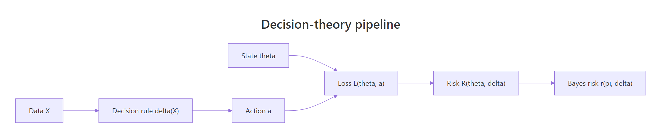
Figure 1: The decision-theory pipeline, data feeds a rule that produces an action, the loss compares the action to the true state, and averaging gives risk and Bayes risk.
Try it: Implement the Huber loss with threshold $k = 1$, which behaves like squared error for small residuals and like absolute error for large ones.
Click to reveal solution
Explanation: Inside the band $|r|\le k$ the loss is quadratic; outside, it switches to linear so a few large outliers do not dominate the optimisation.
How do you compute the risk function in R?
The risk $R(\theta, \delta) = E_\theta\,[\,L(\theta, \delta(X))\,]$ is the expected loss when the data come from $\theta$ and we use rule $\delta$. We can never measure it from one dataset, but we can estimate it cheaply by Monte Carlo: simulate many datasets at a fixed $\theta$, apply the rule, average the loss. Repeat across a $\theta$ grid to get the whole risk function.
Across the grid the simulated risk hovers near $0.04 = 1/25$. That matches the closed-form result $R(\mu, \bar X) = \sigma^2 / n$, which does not depend on $\mu$ at all, the risk is flat. A flat risk function will turn out to be the key to the minimax property later. Now compare with a shrinkage rule $\delta_c(X) = c\bar X$ that pulls the estimate towards zero.
compute_risk general.The shrinkage rule beats the MLE near $\mu = 0$ (lower variance) but its risk grows as $\mu^2$ once you move away, a classic bias-variance trade. No single rule dominates everywhere; that is exactly the situation that motivates Bayes risk and admissibility next.
Try it: Use compute_risk to estimate the risk of the constant rule $\delta_0(X) = 0$ across mu_grid. You should see a parabola.
Click to reveal solution
Explanation: The constant rule has zero variance but bias $\mu$, so its risk is $\mu^2$, a perfect parabola.
What is Bayes risk and when is it minimised?
Risk is a function of $\theta$, so two rules can swap places as $\theta$ moves. To collapse the comparison to a single number, average the risk against a prior $\pi(\theta)$. The result is the Bayes risk $r(\pi, \delta) = \int R(\theta, \delta)\,\pi(\theta)\,d\theta$. The rule that minimises Bayes risk is the Bayes rule, and under squared loss the Bayes rule is the posterior mean.
We will demonstrate with a Beta-Binomial setup: $X \sim \text{Bin}(n, \theta)$, prior $\theta \sim \text{Beta}(\alpha, \beta)$, posterior $\theta\mid X \sim \text{Beta}(\alpha + X, \beta + n - X)$, so the posterior mean is $(\alpha + X) / (\alpha + \beta + n)$.
For this draw the MLE matches the truth exactly, while the posterior mean is pulled slightly toward the prior centre $0.5$. On any single sample either could be closer to the truth. The point of Bayes risk is to ask which rule wins on average, where the average is over both the data and the prior on $\theta$.
The posterior mean has a smaller Bayes risk than the MLE under this Beta(2,2) prior, about a 23% reduction. That is the Bayes rule earning its name: among all rules, it minimises the prior-weighted average risk. The reduction comes from sharing information across $\theta$ values via the prior, which is why prior choice is itself a modelling decision.
Try it: Replace the Beta(2,2) prior with a more informative Beta(20,20) prior (mean 0.5, much tighter). Recompute the Bayes risk of the posterior mean. It should drop further.
Click to reveal solution
Explanation: A tighter prior pulls posterior means even closer to $\theta$, so the squared error shrinks. The trade-off is that a wrong tight prior would raise risk for $\theta$ values it dis-prefers, Bayes risk averages this away under the prior you actually believe.
When is an estimator admissible?
A rule $\delta$ is inadmissible if some other rule $\delta'$ has $R(\theta, \delta') \le R(\theta, \delta)$ for every $\theta$, with strict inequality for at least one $\theta$. Otherwise $\delta$ is admissible. Admissibility is a minimum bar: an inadmissible rule is dominated everywhere, so you should never use it. The catch is that admissibility says nothing about how good the rule is in absolute terms.
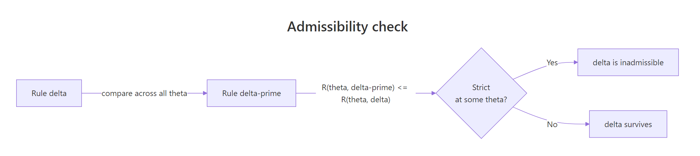
Figure 2: Admissibility check, rule δ is inadmissible if some δ' has equal-or-smaller risk for every θ and strictly smaller for at least one θ.
The clearest demonstration: the constant rule $\delta_0(X) = 0$ has risk $\mu^2$ while the sample mean has constant risk $1/n$. They cross at $\mu = \pm 1/\sqrt n$, so neither dominates the other on the full real line, both are admissible there. But if we restrict the parameter space to $\mu \in [0.5, \infty)$, then sample mean dominates and the constant rule becomes inadmissible.
mean_dominates is TRUE everywhere on the grid, so the sample mean dominates the constant zero rule on $[0.5, 3]$. That makes the constant rule inadmissible there, there is no $\mu$ in this set where it ties or wins. On the full real line the same constant rule is admissible because it beats the sample mean in a neighbourhood of $\mu = 0$, however small.
Try it: Find a single value of $\mu$ where the constant rule $\delta_0$ has lower risk than the sample mean.
Click to reveal solution
Explanation: Within the small neighbourhood $|\mu| < 1/\sqrt n = 0.2$, the constant zero rule beats the sample mean. That neighbourhood is what saves the constant rule from being dominated globally on the whole real line.
How do minimax estimators relate to Bayes estimators?
Minimax shifts focus from averages to worst cases: $\delta^\star$ is minimax if $\sup_\theta R(\theta, \delta^\star) \le \sup_\theta R(\theta, \delta)$ for every other rule $\delta$. The classic theorem says: a Bayes rule whose risk function is constant in $\theta$ is automatically minimax, and the prior making it Bayes is called the least favourable prior.
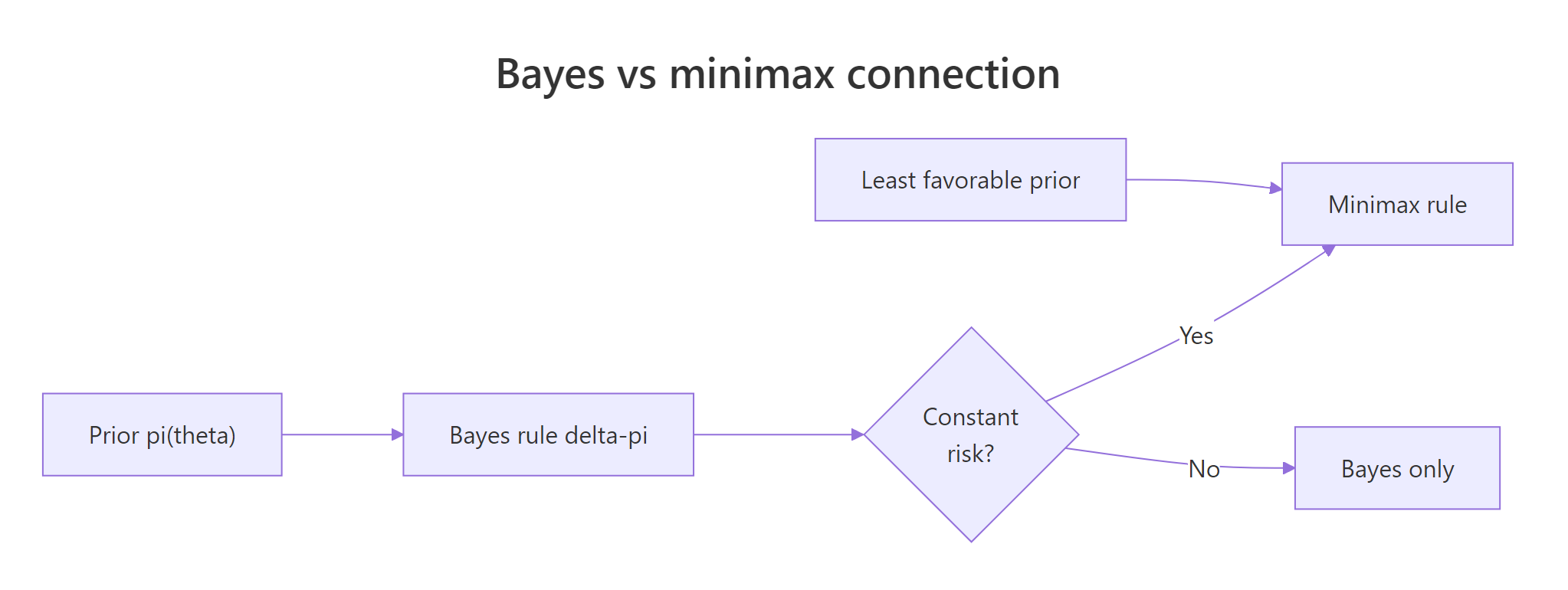
Figure 3: A Bayes rule with constant risk is minimax; the prior that achieves this is called least favourable.
We already saw the sample mean has constant risk $1/n$ for $N(\theta, 1)$. Let us verify and use that to claim it is minimax under squared loss.
The risk stays in a tight band around $1/25 = 0.04$ across a wide $\theta$ range, with simulation noise the only source of variation. So the worst-case risk of the sample mean across all $\mu$ is $\approx 0.04$. Any other rule with a worst-case risk above that cannot be minimax. The sample mean is in fact the unique minimax estimator for the normal mean under squared loss (Lehmann & Casella, Chapter 5).
Try it: Show that the shrinkage rule $\delta_{0.5}(X) = 0.5\bar X$ is not minimax, its risk grows without bound as $|\mu|$ increases.
Click to reveal solution
Explanation: At $\mu = 10$ the rule's bias is $-5$, so its risk $\approx 25$ blows up. The supremum is unbounded, so it cannot be minimax, the sample mean's worst case of $0.04$ wins on the whole real line.
Practice Exercises
Exercise 1: Build a generic risk simulator
Write a function my_risk_sim(estimator, theta_grid, n, B) that returns a data frame with columns theta and risk for any estimator under squared loss with $N(\theta, 1)$ data. Use it to compare mean vs c=0.7 shrinkage on seq(-2, 2, by = 0.5). Save the comparison to my_result.
Click to reveal solution
Explanation: The simulator factors out estimator and grid, so swapping rules is one line. Shrinkage wins near $\theta = 0$ but loses badly far from it, neither dominates, both are admissible on $\mathbb{R}$.
Exercise 2: Beta-Binomial Bayes risk reduction
For $X \sim \text{Bin}(n=20, \theta)$ and prior $\theta \sim \text{Beta}(2, 2)$, compute the Bayes risk of the posterior mean and the MLE under squared loss using 5000 Monte Carlo draws each. Report the percentage reduction the posterior mean achieves over the MLE. Save the percentage to my_pct_drop.
Click to reveal solution
Explanation: The posterior mean borrows strength from the prior, so on average over $\theta$ drawn from Beta(2,2) it cuts Bayes risk by about 21%. The reduction would shrink if the prior were misspecified, try a Beta(50,1) prior to see the cost of a wrong, tight prior.
Complete Example
Let us put loss, risk, Bayes risk, and admissibility together in one comparison. We will study four estimators of a Normal mean under squared loss across a $\theta$ grid: the MLE (sample mean), a posterior mean under a $N(0, 1)$ prior, a fixed shrinkage $\delta_{0.6}(X) = 0.6\bar X$, and the constant rule $\delta_0(X) = 0$. The output is a tidy data frame plus a faceted ggplot panel.
The plot reproduces every concept from this tutorial in one picture. The MLE has flat risk $\approx 0.04$ and is minimax. The posterior mean and shrinkage rule beat the MLE near $\mu = 0$ but pay quadratically as $|\mu|$ grows, they are admissible but not minimax. The constant rule is the most extreme version of shrinkage and hugs the floor only at $\mu = 0$. Choose your estimator by deciding which $\mu$ region matters: prior beliefs about $\theta$ determine that, which is exactly why Bayes risk is the tiebreaker.
Summary
| Concept | Definition | R recipe | Optimal under squared loss |
|---|---|---|---|
| Loss | $L(\theta, a)$ | sq_loss <- function(t,a) (t-a)^2 |
mean |
| Risk | $E_\theta L(\theta, \delta(X))$ | compute_risk(estimator, theta) |
depends on $\theta$ |
| Bayes risk | $E_\pi[R(\theta, \delta)]$ | average risk over prior draws | posterior mean |
| Admissibility | not dominated everywhere | check no rule has lower risk for every $\theta$ | varies |
| Minimax | minimum worst-case risk | constant-risk Bayes rule under least-favourable prior | sample mean for $N(\theta,1)$ |
- The loss is a modelling choice. Pick it to match the cost of real mistakes, not for mathematical convenience.
- The risk function is a function of $\theta$, not a number. Rules cross; no single estimator is best everywhere.
- Bayes risk averages risk by your prior. The Bayes rule under squared loss is the posterior mean.
- Admissibility means "not dominated". Easy to disprove, hard to prove, and surprisingly fragile (Stein's paradox in $p \ge 3$).
- Minimax minimises the worst case. Constant-risk Bayes rules are minimax, that's how the two paradigms shake hands.
References
- Lehmann, E. L. & Casella, G., Theory of Point Estimation, 2nd ed. Springer (1998). Chapters 1, 4, 5.
- Berger, J. O., Statistical Decision Theory and Bayesian Analysis, 2nd ed. Springer (1985).
- Wasserman, L., All of Statistics. Chapter 13: Statistical Decision Theory.
- Robert, C., The Bayesian Choice, 2nd ed. Springer (2007). Chapters 2–3.
- Wasserman, L., Lecture Notes 14, 36-705. Link
- Wikipedia, Admissible decision rule. Link
- Wikipedia, Bayes estimator. Link
Continue Learning
- UMVUE in R, minimum-variance unbiased estimators and how the Cramér–Rao bound interacts with admissibility.
- Cramér–Rao Lower Bound in R, risk lower bound that any unbiased estimator must respect.
- Neyman–Pearson Lemma in R, decision theory applied to hypothesis testing, with 0–1 loss reframed as Type I/II errors.