R Factors: The Data Type That Trips Up Almost Every R Beginner

A factor in R is a character vector with two twists: it memorises the set of allowed values (its levels), and it stores each element as a small integer pointing into that lookup. That's why factors plot, dispatch, and sort in ways raw strings don't, and why converting them back to numbers needs two careful steps.

This guide shows what a factor actually is, how to reorder and relabel levels, when to reach for ordered factors, how forcats makes factor surgery painless, and the three classic bugs that ruin beginner analyses.

Why do R factors exist at all?

Before forcats and modern tidyverse, R had factor(), and the reason it exists is statistical modelling. When you fit lm(y ~ group) and group is a character vector, R has to pick which category is the baseline, how to dummy-code the rest, and what to do at prediction time if a new category appears. Factors bake those decisions into the data: a fixed set of allowed levels, a known order, and a compact integer storage.

Let's build one by hand and peek at what's inside. The underlying representation is the whole point.

RFactor is an integer with levels

# A factor is an integer vector wearing a levels hat sizes <- c("small", "large", "medium", "small", "large") f <- factor(sizes) f #> [1] small large medium small large #> Levels: large medium small typeof(f) # what's actually in memory #> [1] "integer" as.integer(f) # the level codes, not the values! #> [1] 3 1 2 3 1 levels(f) # the lookup table #> [1] "large" "medium" "small" class(f) #> [1] "factor"

f prints as words, but typeof(f) says "integer", the factor is storing c(3, 1, 2, 3, 1) and pointing into the alphabetised levels vector c("large", "medium", "small"). That's why as.integer(f) hands you level codes, not the original strings, a beginner trap we'll fix in the gotchas section.

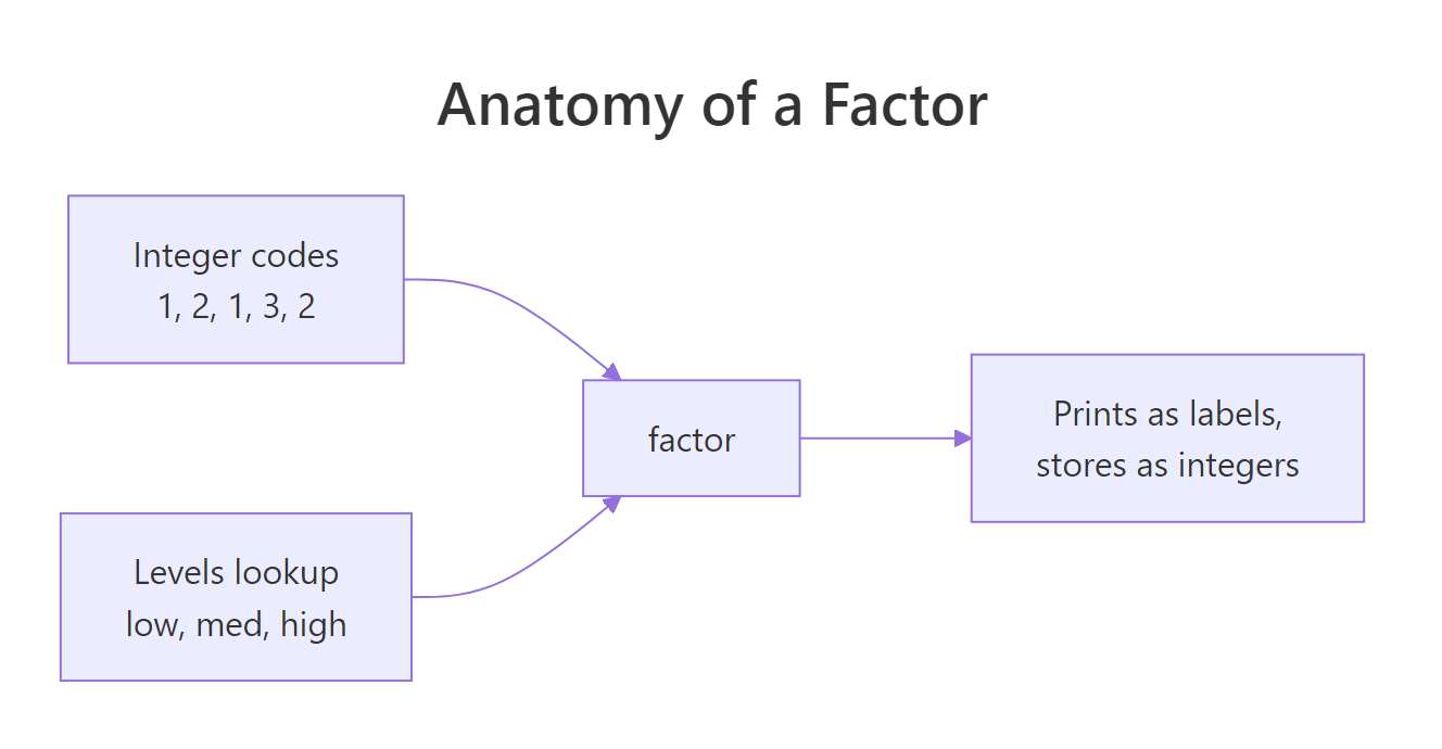
Anatomy of a factor: codes plus levels

Figure 1: A factor is an integer vector plus a levels lookup. The integer codes point into levels; printing and plotting use the string labels.

Try it: Build a factor ex_grade from c("B", "A", "C", "B", "A") and print (a) the underlying integer codes and (b) the levels.

RExercise: grade factor anatomy

# Try it: anatomy of a factor ex_grade <- factor(c("B", "A", "C", "B", "A")) as.integer(ex_grade) #> Expected: [1] 2 1 3 2 1 levels(ex_grade) #> Expected: [1] "A" "B" "C"

Click to reveal solution

RGrade factor solution

ex_grade <- factor(c("B", "A", "C", "B", "A")) as.integer(ex_grade) #> [1] 2 1 3 2 1 levels(ex_grade) #> [1] "A" "B" "C"

Explanation: Levels are alphabetical by default. "A" is level 1, "B" is level 2, "C" is level 3, so the sequence B, A, C, B, A becomes the integer codes 2, 1, 3, 2, 1.

How do you control the order of factor levels?

The default order is alphabetical, which is almost never what you want. "Low / Medium / High" should be in that order on a plot axis. "Monday / Tuesday / ... / Sunday" should be chronological. Controlling level order is where factors earn their keep, and there are four ways to do it, two in base R, two in forcats.

Ordered vs unordered factors

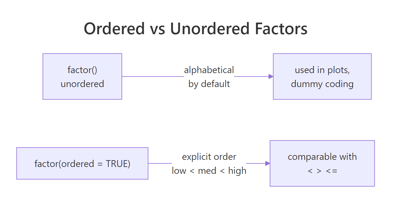
Figure 2: Unordered factors have a level sequence used for plots and model coding but can't be compared with <. Ordered factors add comparisons and use polynomial contrasts in models.

RFour ways to control level order

# Four ways to control level order x <- c("high", "low", "medium", "low", "high", "medium") # 1. factor(..., levels = ...), set order at creation f1 <- factor(x, levels = c("low", "medium", "high")) levels(f1) #> [1] "low" "medium" "high" # 2. Reorder existing factor with factor() f0 <- factor(x) f2 <- factor(f0, levels = c("low", "medium", "high")) levels(f2) #> [1] "low" "medium" "high" # 3. forcats::fct_relevel, cleaner API library(forcats) f3 <- fct_relevel(f0, "low", "medium", "high") levels(f3) #> [1] "low" "medium" "high" # 4. Data-driven reorder: fct_infreq (most frequent first) f4 <- fct_infreq(f0) levels(f4) #> [1] "high" "low" "medium"

factor(x, levels = ...) at creation time is the idiom to learn first, it documents the intended order right next to the data. fct_relevel() is the cleanest for modifying an existing factor, and fct_infreq() / fct_inorder() handle the common cases of "most common first" and "order of appearance" without you having to type the levels out.

Tip

Set levels at creation, not after the fact. The moment you know the allowed categories and their order, write factor(x, levels = c(...)). Fixing level order in a downstream step (especially after subsetting) invites silent bugs where missing categories get dropped.

Try it: Turn ex_days <- c("Wed", "Mon", "Fri", "Tue", "Thu") into a factor whose levels are ordered Mon, Tue, Wed, Thu, Fri.

RExercise: chronological day factor

# Try it: chronological day order ex_days <- c("Wed", "Mon", "Fri", "Tue", "Thu") ex_f <- NULL # your code here levels(ex_f) #> Expected: [1] "Mon" "Tue" "Wed" "Thu" "Fri"

Click to reveal solution

RChronological day solution

ex_days <- c("Wed", "Mon", "Fri", "Tue", "Thu") ex_f <- factor(ex_days, levels = c("Mon","Tue","Wed","Thu","Fri")) levels(ex_f) #> [1] "Mon" "Tue" "Wed" "Thu" "Fri"

Explanation: Passing levels = at creation time locks the order. The underlying integer codes are chosen to match this ordering, so plots and tables will show the days in chronological order.

When should you use an ordered factor?

An ordered factor (ordered = TRUE) adds one thing: you can compare its elements with <, >, <=, >=. factor("low") < factor("high") throws a warning and returns NA, but ordered("low", levels = c("low","med","high")) < ordered("high", ...) is TRUE.

Ordered factors are the right choice for genuine ordinal variables, survey responses (strongly disagree < disagree < neutral < agree < strongly agree), clinical stages, letter grades. They also change how lm() dummy-codes the variable: ordered factors get polynomial contrasts by default, which you may or may not want.

ROrdered factor enables comparison

# Ordered factor unlocks comparison ord <- factor(c("low","high","med","low"), levels = c("low","med","high"), ordered = TRUE) ord #> [1] low high med low #> Levels: low < med < high ord[1] < ord[2] # TRUE, low < high #> [1] TRUE ord[1] < ord[3] # TRUE, low < med #> [1] TRUE max(ord) # "high" #> [1] high #> Levels: low < med < high # Compare to unordered, comparison fails with a warning un <- factor(c("low","high","med","low"), levels = c("low","med","high")) un[1] < un[2] #> Warning: '<' not meaningful for factors #> [1] NA

The printed Levels: low < med < high line is how you spot an ordered factor at a glance, the < separator means "these are comparable". max(ord) returns "high" because high has the greatest level code, which is what you want for ordinal data.

Note

Ordered factors change model contrasts. When you fit lm(y ~ ord_factor), R uses polynomial contrasts (linear, quadratic, ...) instead of dummy coding. If you just want level 1 as the baseline and dummies for the rest, either use an unordered factor or set contrasts = list(ord_factor = contr.treatment) explicitly.

Try it: Build an ordered factor ex_tee from c("M","XL","S","L") with the size order S < M < L < XL, then return the smallest value with min().

RExercise: ordered tee-shirt sizes

# Try it: ordered factor + min ex_tee <- NULL # your code here min(ex_tee) #> Expected: [1] S #> Levels: S < M < L < XL

Click to reveal solution

RTee-shirt size solution

ex_tee <- factor(c("M","XL","S","L"), levels = c("S","M","L","XL"), ordered = TRUE) min(ex_tee) #> [1] S #> Levels: S < M < L < XL

Explanation: ordered = TRUE tells R the levels argument defines a genuine ordering. min() returns the element with the smallest level code, S, which is level 1.

How does forcats make factor work painless?

forcats (a tidyverse package loaded by library(tidyverse)) is built around one observation: almost every operation on a factor is "move levels around", "rename them", or "collapse rare ones", and base R's API for each is clunky. forcats gives every operation a clear fct_*() name and keeps the factor structure intact.

The six you'll use most are fct_relevel, fct_recode, fct_collapse, fct_lump, fct_reorder, and fct_drop. They solve 90% of factor chores in one line each.

Rforcats: reorder, rename, collapse

library(forcats) fruit <- factor(c("apple","banana","apple","cherry","durian","apple","banana","kiwi")) # Reorder by count (most frequent first) fct_infreq(fruit) #> [1] apple banana apple cherry durian apple banana kiwi #> Levels: apple banana cherry durian kiwi # Rename levels fct_recode(fruit, Apple = "apple", Banana = "banana") #> [1] Apple Banana Apple cherry durian Apple Banana kiwi #> Levels: Apple Banana cherry durian kiwi # Collapse several levels into one fct_collapse(fruit, tropical = c("banana", "durian", "kiwi")) #> [1] apple tropical apple cherry tropical apple tropical tropical #> Levels: apple tropical cherry # Lump rare levels into "Other" fct_lump(fruit, n = 2) # keep top 2, rest -> Other #> [1] apple banana apple Other Other apple banana Other #> Levels: apple banana Other # Drop unused levels after subsetting sub <- fruit[fruit %in% c("apple","banana")] levels(sub) # still has all 5 levels, annoying #> [1] "apple" "banana" "cherry" "durian" "kiwi" fct_drop(sub) # now only the ones that appear #> [1] apple banana apple apple banana #> Levels: apple banana

Each function takes a factor and returns a new factor, nothing mutates in place, and chains with |> compose beautifully. fct_lump() and fct_collapse() are the big time-savers when your category column has a long tail of rare values you want bundled as "Other".

Warning

Subsetting a factor keeps unused levels. fruit[fruit == "apple"] still has "banana", "cherry", and the rest in its levels, which shows up as empty bars on plots and empty rows in tables. Always follow a subset with droplevels() or fct_drop() if you don't want the ghosts.

Try it: Use forcats to relabel the fruit factor so "apple" and "kiwi" both become "green" and everything else becomes "other".

RExercise: collapse with fctcollapse

# Try it: collapse with fct_collapse library(forcats) ex_grouped <- NULL # your code here levels(ex_grouped) #> Expected: [1] "green" "other" (plus any other remaining levels)

Click to reveal solution

Rfctcollapse solution

library(forcats) ex_grouped <- fct_collapse(fruit, green = c("apple", "kiwi"), other = c("banana", "cherry", "durian")) ex_grouped #> [1] green other green other other green other green #> Levels: green other levels(ex_grouped) #> [1] "green" "other"

Explanation: fct_collapse() maps a set of old levels to each new level. Any level not mentioned stays as-is, so listing every bucket keeps the output tidy.

What are the three classic factor gotchas?

Three bugs account for most factor pain. Each one has a specific fix, and once you've seen them, you'll never fall for them again.

RThree classic factor gotchas

# Gotcha 1: as.numeric(factor) returns the codes, not the labels years <- factor(c("2020","2021","2019","2021")) as.numeric(years) #> [1] 2 3 1 3 # codes, NOT the year values! as.numeric(as.character(years)) #> [1] 2020 2021 2019 2021 # correct two-step # Gotcha 2: adding a value outside the allowed levels fr <- factor(c("yes","no","yes"), levels = c("yes","no")) fr[4] <- "maybe" #> Warning: invalid factor level, NA generated fr #> [1] yes no yes <NA> # Fix: expand the levels first levels(fr) <- c(levels(fr), "maybe") fr[4] <- "maybe" fr #> [1] yes no yes maybe #> Levels: yes no maybe # Gotcha 3: combining two factors with c() discards labels a <- factor(c("x","y")) b <- factor(c("y","z")) c(a, b) # pre-R 4.1 returns integers! #> [1] x y y z # R 4.1+ stitches levels, but be explicit: #> Levels: x y z # Explicit and safe across versions factor(c(as.character(a), as.character(b))) #> [1] x y y z #> Levels: x y z

Gotcha 1, as.numeric(factor), is the single most destructive. If you load a CSV where a year column came in as a factor and write mean(df$year), you get the mean of the level codes, which looks like a plausible small number and is completely wrong. The fix is always as.numeric(as.character(x)), or better, ensure the column never becomes a factor by using stringsAsFactors = FALSE (the default in R 4.0+).

Warning

as.numeric(factor) returns level codes, not label values. Always use as.numeric(as.character(f)) when the factor labels are strings of digits. The first form silently returns 1, 2, 3, ... instead of 2019, 2020, 2021, ..., and the bug is almost impossible to spot in a summary statistic.

Try it: ex_yr <- factor(c("2030","2028","2029","2028")). Compute the correct mean of the years using the two-step idiom.

RExercise: mean of a year factor

# Try it: mean of a year factor ex_yr <- factor(c("2030","2028","2029","2028")) ex_mean <- NULL # your code here ex_mean #> Expected: 2028.75

Click to reveal solution

RYear-factor mean solution

ex_yr <- factor(c("2030","2028","2029","2028")) ex_mean <- mean(as.numeric(as.character(ex_yr))) ex_mean #> [1] 2028.75

Explanation: as.character(ex_yr) rebuilds the strings "2030","2028","2029","2028". as.numeric() then parses them to doubles. Without as.character() you'd get the mean of the level codes c(3,1,2,1), about 1.75, which is silently wrong.

Practice Exercises

Two capstone exercises that combine factor creation, reordering, and level hygiene.

Exercise 1: Chronological month factor

Given my_months <- c("Mar","Jan","Feb","Mar","Jan","Dec"), build my_fac as a factor whose levels are the twelve months in chronological order ("Jan" through "Dec"). Then run droplevels() to get a version that contains only the months that actually appear.

RExercise: chronological factor with hygiene

# Exercise 1: chronological factor with clean levels my_months <- c("Mar","Jan","Feb","Mar","Jan","Dec") my_fac <- NULL my_trim <- NULL levels(my_fac) #> Expected: all 12 month abbreviations in order levels(my_trim) #> Expected: [1] "Jan" "Feb" "Mar" "Dec"

Click to reveal solution

RChronological factor solution

my_months <- c("Mar","Jan","Feb","Mar","Jan","Dec") month_levels <- c("Jan","Feb","Mar","Apr","May","Jun", "Jul","Aug","Sep","Oct","Nov","Dec") my_fac <- factor(my_months, levels = month_levels) my_trim <- droplevels(my_fac) levels(my_fac) #> [1] "Jan" "Feb" "Mar" "Apr" "May" "Jun" "Jul" "Aug" "Sep" "Oct" "Nov" "Dec" levels(my_trim) #> [1] "Jan" "Feb" "Mar" "Dec"

Explanation: Passing all 12 months to levels locks the chronological order even though the data only contains 4 of them. droplevels() then strips the unused levels, essential before plotting so empty months don't show up as gaps.

Exercise 2: Safe factor-to-numeric with forcats

Given my_score <- factor(c("85","72","91","72","60")), build my_num, the numeric vector of the same scores, and my_lumped, a new factor where scores below 80 are recoded to "low" and scores 80+ are "high". Use forcats::fct_collapse for the second part.

RExercise: convert and collapse scores

# Exercise 2: convert and collapse library(forcats) my_score <- factor(c("85","72","91","72","60")) my_num <- NULL my_lumped <- NULL my_num #> Expected: [1] 85 72 91 72 60 my_lumped #> Expected: levels "low" "high"

Click to reveal solution

RConvert-and-collapse solution

library(forcats) my_score <- factor(c("85","72","91","72","60")) my_num <- as.numeric(as.character(my_score)) low_labels <- levels(my_score)[as.numeric(levels(my_score)) < 80] high_labels <- levels(my_score)[as.numeric(levels(my_score)) >= 80] my_lumped <- fct_collapse(my_score, low = low_labels, high = high_labels) my_num #> [1] 85 72 91 72 60 my_lumped #> [1] high low high low low #> Levels: low high

Explanation: as.numeric(as.character(my_score)) is the correct two-step for converting a numeric-labelled factor. fct_collapse() then groups the original level labels into "low" and "high" buckets. Building the two label groups from levels(my_score) makes the collapse rule data-driven instead of hard-coded.

Complete Example

A small end-to-end flow that simulates survey data, cleans the categorical column, fixes the level order, and feeds the result to table() and barplot(), no downstream surprises.

REnd-to-end survey factor cleanup

# Complete example: survey responses -> plot-ready factor set.seed(42) responses <- sample( c("strongly agree", "agree", "neutral", "disagree", "strongly disagree", "no answer"), size = 30, replace = TRUE, prob = c(0.15, 0.25, 0.20, 0.15, 0.10, 0.15) ) # Step 1: fix the level order explicitly (Likert scale) likert_levels <- c("strongly disagree","disagree","neutral","agree","strongly agree") resp_fac <- factor(responses, levels = c(likert_levels, "no answer")) table(resp_fac) #> resp_fac #> strongly disagree disagree neutral agree #> 1 4 7 8 #> strongly agree no answer #> 5 5 # Step 2: treat "no answer" as NA library(forcats) resp_clean <- fct_recode(resp_fac, NULL = "no answer") table(resp_clean, useNA = "ifany") #> resp_clean #> strongly disagree disagree neutral agree #> 1 4 7 8 #> strongly agree <NA> #> 5 5 # Step 3: as.ordered for comparisons resp_ord <- factor(as.character(resp_clean), levels = likert_levels, ordered = TRUE) min(resp_ord, na.rm = TRUE) #> [1] strongly disagree #> Levels: strongly disagree < disagree < neutral < agree < strongly agree # Step 4: counts for plotting counts <- table(resp_ord) counts #> resp_ord #> strongly disagree disagree neutral agree #> 1 4 7 8 #> strongly agree #> 5

The full pipeline: lock the Likert order at creation, recode the sentinel "no answer" to NA, upgrade to ordered for semantically correct comparisons, and feed a clean table() into a plotting function. Every step is a one-liner once you know the forcats vocabulary.

Summary

Concept	One-line takeaway
A factor is	an integer vector pointing into a `levels` character lookup
Default order	alphabetical, override with `factor(x, levels = ...)`
Ordered factor	adds `<` comparisons and polynomial contrasts in `lm()`
forcats verbs	`fct_relevel`, `fct_recode`, `fct_collapse`, `fct_lump`, `fct_drop`
Subsetting	keeps unused levels, follow with `droplevels()`
Biggest bug	`as.numeric(factor)` returns level codes, not labels, use `as.numeric(as.character(f))`

Key Insight

Factors are not strings in a hat, they're integer vectors with a lookup table and a class attribute. Once that clicks, every quirk (the two-step conversion, the subset level-retention, the ordered-factor contrasts) becomes a logical consequence instead of an arbitrary rule. For interactive work, prefer forcats verbs; for modelling, be deliberate about whether your factor is ordered.

References

Wickham, H. Advanced R (2nd ed.), §3.5 Augmented vectors, Factors. adv-r.hadley.nz/vectors-chap.html#factors
Wickham, H. and Grolemund, G. R for Data Science, Chapter 15: Factors with forcats. r4ds.had.co.nz/factors.html
forcats package documentation. forcats.tidyverse.org
R documentation: ?factor, ?levels, ?droplevels, ?contrasts.
R news: stringsAsFactors default changed to FALSE in R 4.0.0. stat.ethz.ch/pipermail/r-announce/2020/000653.html
R Core Team. An Introduction to R, §4 Ordered and unordered factors.

Continue Learning

R Data Types: Which Type Is Your Variable?, The parent post on R's atomic types, of which factor is the most commonly misused augmented variant.
R Type Coercion: Why Your Numeric Columns Silently Turn Into Characters, The coercion rules that turn factor → numeric into a two-step operation.
R Attributes: The Hidden Metadata That Makes R Objects Behave Differently, Factors are a textbook example of the "integer vector + class attribute + levels attribute" pattern.

R Factors: The Data Type That Trips Up Almost Every R Beginner

Why do R factors exist at all?

How do you control the order of factor levels?

When should you use an ordered factor?

How does forcats make factor work painless?

What are the three classic factor gotchas?

Practice Exercises

Exercise 1: Chronological month factor

Exercise 2: Safe factor-to-numeric with forcats

Complete Example

Summary

References

Continue Learning

Related Tutorials