Hypothesis Testing in R: Understand the Framework, Not Just the p-Value

Hypothesis testing is a structured decision rule for asking, "Is this pattern in my data real, or could it have appeared by chance?", and R gives you one consistent toolkit (t.test(), prop.test(), chisq.test(), and friends) for running it.

What is the hypothesis testing framework?

Most tutorials hand you a p-value and tell you "less than 0.05 means significant." That hides the actual machinery. Hypothesis testing is a five-step decision process: pick two competing claims, summarise your data into a single number, ask how surprising that number is if the boring claim were true, then decide. We'll run the whole loop in one block on the mtcars dataset, then unpack each step in the sections that follow.

Here is a complete one-sample t-test asking, "Is the average miles-per-gallon of the 32 cars in mtcars different from 20?" Watch the output, every later section explains one piece of it.

ROne-sample t-test on mtcars mpg

# Five-step hypothesis test in one block # H0: mean mpg = 20 H1: mean mpg != 20 payoff_test <- t.test(mtcars$mpg, mu = 20) payoff_test #> One Sample t-test #> #> data: mtcars$mpg #> t = 0.08506, df = 31, p-value = 0.9328 #> alternative hypothesis: true mean is not equal to 20 #> 95 percent confidence interval: #> 17.91768 22.26357 #> sample estimates: #> mean of x #> 20.09062 # Plain-English decision if (payoff_test$p.value < 0.05) { "Reject H0, mean mpg differs from 20." } else { "Fail to reject H0, no evidence mean mpg differs from 20." } #> [1] "Fail to reject H0, no evidence mean mpg differs from 20."

The sample mean (20.09) is essentially on top of our hypothesised 20, the t statistic is tiny (0.085), and the p-value of 0.93 says "this difference is exactly the kind of thing you'd see all the time if H₀ were true." So we keep H₀. Notice we never proved H₀, we only failed to find evidence against it. That phrasing matters and we'll come back to it.

Key Insight

Every p-value is computed assuming H₀ is true. It's the answer to "if the boring claim held, how often would I see data this extreme?", never "what's the probability the null is true?" Get that one sentence right and 90% of statistics misreporting disappears.

Try it: Re-run the same test against mu = 25 instead of 20. Predict before running: do you expect the p-value to go up or down?

RExercise: predict p-value at mu 25

# Try it: change mu and predict the direction ex_test <- t.test(mtcars$mpg, mu = ___) # replace ___ with 25 ex_test$p.value #> Expected: a much smaller p-value (well below 0.05)

Click to reveal solution

RMu-25 solution

ex_test <- t.test(mtcars$mpg, mu = 25) ex_test$p.value #> [1] 7.139703e-06

Explanation: The sample mean of 20.09 is far from 25 relative to its standard error, so the t statistic is large and the tail probability is tiny. We now have strong evidence to reject H₀.

How do you state the null and alternative hypothesis?

The null hypothesis (H₀) is always the boring, conservative claim, no difference, no effect, no relationship. The alternative hypothesis (H₁) is what you'd accept if the data forces you off H₀. You write them down before you look at the data, because the framework only makes sense when H₀ is the default you'd cling to without evidence.

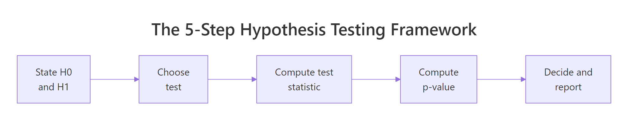
The five-step decision loop every hypothesis test follows.

Figure 1: The five-step decision loop every hypothesis test follows.

Let's compare 4-cylinder and 6-cylinder cars in mtcars. The question is whether their mean mpg differs. H₀: μ₄ = μ₆. H₁: μ₄ ≠ μ₆. The ~ formula in t.test() says "split mpg by cyl group."

RTwo-sample Welch t-test by cyl

# Two-sample t-test, two-sided # H0: mean mpg is the same in 4-cyl and 6-cyl groups cars_4_6 <- subset(mtcars, cyl %in% c(4, 6)) t.test(mpg ~ cyl, data = cars_4_6) #> Welch Two Sample t-test #> #> data: mpg by cyl #> t = 4.7191, df = 12.956, p-value = 0.0004048 #> alternative hypothesis: true difference in means between group 4 and group 6 is not equal to 0 #> 95 percent confidence interval: #> 3.751376 9.929907 #> sample estimates: #> mean in group 4 mean in group 6 #> 26.66364 19.74286

The mean mpg gap is about 6.9 mpg, the t statistic is 4.7, and the p-value is 0.0004. That p-value says: "if 4-cyl and 6-cyl cars truly had the same mean mpg, you'd see a gap this big or bigger less than 1 time in 2,000." That's surprising enough to reject H₀.

Now suppose your scientific question was specifically directional: "Do 4-cyl cars have higher mpg than 6-cyl?" You'd use a one-sided test. R defaults to two-sided; switch with alternative = "greater".

ROne-sided alternative greater

# One-sided alternative: 4-cyl > 6-cyl cars_4_6_one <- t.test(mpg ~ cyl, data = cars_4_6, alternative = "greater") cars_4_6_one$p.value #> [1] 0.0002023776

The one-sided p-value is exactly half the two-sided value because the t distribution is symmetric, we're now only counting the right tail. One-sided tests have more power when the direction is genuinely pre-specified, but they're easy to abuse.

Warning

Never pick a one-sided test after peeking at the data direction. If you eyeball the sample, see 4-cyl is higher, then declare your alternative, you've effectively doubled your false-positive rate. The direction has to come from the scientific question (theory, prior literature, registered analysis plan), not from the sample.

Try it: Write H₀ and H₁ for "do automatic and manual cars (am = 0 vs 1) differ in mpg?" Then run the two-sided t-test and report the decision at α = 0.05.

RExercise: t-test mpg by transmission

# Try it: am vs mpg # H0: ____________________ # H1: ____________________ ex_am <- t.test(mpg ~ am, data = mtcars) ex_am$p.value #> Expected: a small p-value, leading to "reject H0"

Click to reveal solution

H₀: mean mpg is the same for automatic and manual transmissions (μ_auto = μ_manual). H₁: the means differ.

RTransmission solution

ex_am <- t.test(mpg ~ am, data = mtcars) ex_am$p.value #> [1] 0.001373638

Explanation: p ≈ 0.0014 is well below 0.05, so we reject H₀ and conclude the two transmission types have different mean mpg in this dataset.

What is a test statistic and why does it matter?

A test statistic compresses your entire dataset into a single number whose distribution is known under H₀. That known distribution is what lets you turn the number into a p-value. For the one-sample t-test the statistic is:

$$t = \frac{\bar{x} - \mu_0}{s / \sqrt{n}}$$

Where:

$\bar{x}$ is the sample mean
$\mu_0$ is the hypothesised value (the H₀ claim)
$s$ is the sample standard deviation
$n$ is the sample size

The numerator is the raw distance between the sample and H₀. The denominator, the standard error of the mean, is how much that distance would fluctuate just from random sampling. Dividing by it expresses the gap "in standard-error units." A t of 2 means "twice as far from H₀ as random noise would typically push you."

Let's compute the t statistic by hand from mtcars$mpg against μ₀ = 20 and confirm it matches t.test().

RManual t statistic vs t.test

# Manual t statistic vs t.test() x <- mtcars$mpg n <- length(x) xbar <- mean(x) s <- sd(x) mu0 <- 20 t_manual <- (xbar - mu0) / (s / sqrt(n)) t_manual #> [1] 0.08506046 t_obj <- t.test(x, mu = mu0) t_obj$statistic #> t #> 0.08506046

The two numbers agree exactly. The mean (20.09) sits 0.085 standard errors away from 20, a hair's breadth, statistically speaking. That's why the test refuses to reject H₀.

Tip

The denominator is the standard error of the mean, and bigger n shrinks it. Doubling your sample size cuts the SE by a factor of √2 ≈ 1.41, which roughly halves the p-value when the effect is real. This is why "collect more data" is often the right answer to a borderline result.

Try it: Compute the t statistic by hand for iris$Sepal.Length against μ₀ = 5.5, then verify with t.test().

RExercise: manual t for sepal length

# Try it: manual t for iris ex_x <- iris$Sepal.Length # your code: compute ex_t manually using mean, sd, length # Verify: t.test(ex_x, mu = 5.5)$statistic #> Expected: ex_t matches the t.test() value

Click to reveal solution

RSepal-length solution

ex_x <- iris$Sepal.Length ex_t <- (mean(ex_x) - 5.5) / (sd(ex_x) / sqrt(length(ex_x))) ex_t #> [1] 5.078072 t.test(ex_x, mu = 5.5)$statistic #> t #> 5.078072

Explanation: The sample mean (5.84) is roughly 5 standard errors above 5.5, so a one-sample t-test would strongly reject H₀: μ = 5.5.

What does the p-value really mean (and what doesn't it)?

The p-value is the answer to one specific question:

$$p = P(|T| \geq |t_{obs}| \mid H_0)$$

In words: "If H₀ were true, how often would the test statistic land at least as extreme as the value I just computed?" It's a tail-area probability under the null distribution. Nothing more, nothing less.

You can compute it yourself from the t statistic. For a two-sided test, find the area in both tails beyond |t| of the t distribution with n − 1 degrees of freedom.

RManual two-sided p-value via pt

# Manual two-sided p-value via pt() t_val <- t_obj$statistic # from previous block: 0.08506046 df <- n - 1 # 31 p_manual <- 2 * pt(-abs(t_val), df = df) unname(p_manual) #> [1] 0.9327503 t_obj$p.value #> [1] 0.9327503

Identical, as it must be. The p-value isn't magic, it's a direct lookup against a known distribution.

To make the conditional-probability definition concrete, here's a simulation: draw 10,000 datasets where H₀ truly holds (samples from N(0, 1) tested against μ₀ = 0), run a t-test on each, and look at the resulting p-values. If the p-value really is "a tail probability under H₀," its distribution should be uniform on [0, 1].

Rp-value uniformity under H0

# Simulation: distribution of p-values when H0 is true set.seed(2024) null_pvals <- replicate(10000, { s <- rnorm(20, mean = 0, sd = 1) t.test(s, mu = 0)$p.value }) # Should be roughly uniform: ~5% below 0.05, ~10% below 0.10, etc. mean(null_pvals < 0.05) #> [1] 0.0489 mean(null_pvals < 0.10) #> [1] 0.1006 mean(null_pvals < 0.50) #> [1] 0.4994 hist(null_pvals, breaks = 20, col = "lightblue", main = "p-values under H0 (true null)", xlab = "p-value")

About 4.89% of p-values fall below 0.05, exactly what "5% false-positive rate at α = 0.05" means. The histogram is flat, not piled near zero. A flat null distribution is the whole reason p < 0.05 means anything: under H₀ it almost never happens, so when you see it you have grounds to reject.

Warning

Three p-value misreads to retire forever. (1) "p = 0.04 means H₀ has only a 4% chance of being true", wrong, the p-value never tells you the probability of H₀. (2) "p = 0.6 means H₀ is true", wrong, large p just means not enough evidence; the truth could go either way. (3) "p < 0.05 means the effect is large", wrong, p values shrink with sample size; a tiny effect with n = 100,000 will be "significant" but trivial.

Try it: Predict the proportion of simulated p-values that fall below 0.10 when H₀ is true, then verify by running the simulation.

RExercise: predict fraction below 0.10

# Try it: predict, then check # Prediction: about ___% of p-values fall below 0.10 mean(null_pvals < 0.10) #> Expected: very close to 10%

Click to reveal solution

RTen-percent solution

# Under H0, p-values are uniform on [0,1], so P(p < 0.10) ≈ 0.10 mean(null_pvals < 0.10) #> [1] 0.1006

Explanation: A uniform-on-[0,1] distribution puts probability c in any interval of length c, so the fraction of p-values below 0.10 should sit near 10%. The simulation confirms it, and this is the full mechanism behind why fixed α controls false-positive rate.

How do you make a decision and avoid Type I and Type II errors?

The decision rule is simple: pick a significance level α (typically 0.05) before you see the data, then reject H₀ if p < α. There are exactly two ways to be wrong, and they cost you different things.

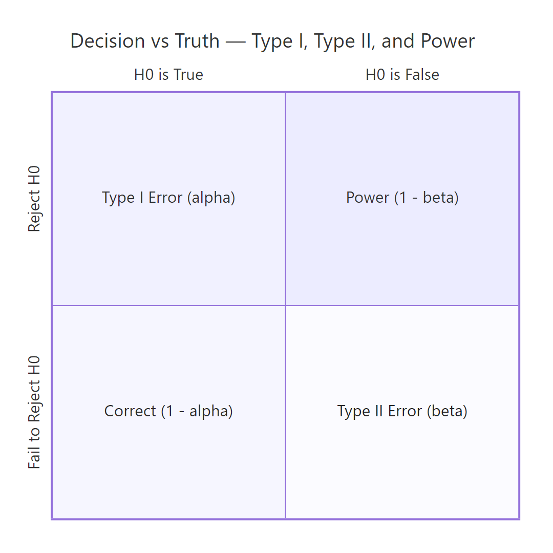
Type I and Type II errors arise from the four cells of decision × truth.

Figure 2: Type I and Type II errors arise from the four cells of decision × truth.

A Type I error is rejecting H₀ when it's actually true, a false positive. Its long-run rate equals α, by construction. A Type II error is failing to reject H₀ when H₁ is true, a false negative, with rate β. Power = 1 − β is the probability of correctly rejecting a false H₀; it depends on the true effect size, the sample size, and α.

Let's verify the Type I rate empirically. Simulate 1,000 t-tests under H₀ and count the false positives.

RType I error rate simulation

# Type I error rate simulation set.seed(42) type1_rejects <- replicate(1000, { s <- rnorm(30, mean = 0, sd = 1) # H0 is true t.test(s, mu = 0)$p.value < 0.05 }) mean(type1_rejects) #> [1] 0.052

Roughly 5.2% of tests rejected even though H₀ was true. That's α in action, it's the price you pay for the ability to ever reject anything.

Now power. Simulate the same test but with a true mean of 0.5 (so H₀: μ = 0 is false) and count the correct rejections.

RPower simulation at true mean 0.5

# Power simulation: true mean = 0.5, H0: mu = 0 set.seed(42) power_rejects <- replicate(1000, { s <- rnorm(30, mean = 0.5, sd = 1) # H1 is true t.test(s, mu = 0)$p.value < 0.05 }) mean(power_rejects) #> [1] 0.756

About 76% of tests correctly rejected H₀, that's our empirical power. The other 24% missed a real effect. Power goes up with sample size, with bigger true effects, and with looser α.

Note

α is your tolerance for false positives, picked by you. The 0.05 default is convention, not law. For drug approvals or fraud detection where false positives are expensive, use 0.01 or smaller. For exploratory analyses where you'd rather investigate too much than miss things, 0.10 is defensible, as long as you state it up front and report it honestly.

Try it: Re-run the power simulation with n = 50 (instead of 30). Predict before running: does power go up or down?

RExercise: power at sample size 50

# Try it: predict, then run ex_power <- replicate(1000, { ex_s <- rnorm(___, mean = 0.5, sd = 1) # n = 50 t.test(ex_s, mu = 0)$p.value < 0.05 }) mean(ex_power) #> Expected: higher than the n=30 case (~0.76)

Click to reveal solution

Rn-50 power solution

set.seed(42) ex_power <- replicate(1000, { ex_s <- rnorm(50, mean = 0.5, sd = 1) t.test(ex_s, mu = 0)$p.value < 0.05 }) mean(ex_power) #> [1] 0.937

Explanation: Bigger n shrinks the standard error, which inflates the t statistic for the same true effect, which pushes more tests into the rejection region. Power rose from ~0.76 (n=30) to ~0.94 (n=50).

How do you choose the right test for your data?

Test choice is dictated by the data structure and the question, not preference. A short decision tree covers most everyday cases:

Data you have	Question	R function
One numeric variable	Differs from a fixed value?	`t.test(x, mu = ...)`
Two numeric groups (independent)	Means differ?	`t.test(x ~ group)`
Two numeric vectors (paired)	Mean difference ≠ 0?	`t.test(x, y, paired = TRUE)`
One proportion	Differs from a fixed value?	`prop.test()` or `binom.test()`
Two categorical variables	Independent?	`chisq.test()` or `fisher.test()`
Numeric, non-normal, small n	Distributions differ?	`wilcox.test()`

Here's one call to each of four common tests, on appropriate data, so you can see the consistent output structure.

RFour common tests, one interface

# Four tests, one consistent interface t_demo <- t.test(extra ~ group, data = sleep) # paired/group means prop_demo <- prop.test(x = c(45, 60), n = c(100, 100)) # two proportions chi_demo <- chisq.test(table(mtcars$cyl, mtcars$am)) # categorical independence wilcox_demo <- wilcox.test(extra ~ group, data = sleep) # non-parametric two-group t_demo$p.value #> [1] 0.07939414 prop_demo$p.value #> [1] 0.04417134 chi_demo$p.value #> [1] 0.01264823 wilcox_demo$p.value #> [1] 0.06932818

Notice every result object exposes $p.value, $statistic, and (for most) $conf.int. Once you've internalised the interface for one test, the rest follow the same shape.

Key Insight

Every R test function returns a list with the same key fields: statistic, p.value, parameter, conf.int. This is not a coincidence, it's a deliberate design that lets you write generic reporting code. extract_results <- function(test) c(test$statistic, p = test$p.value) works on t.test, wilcox.test, chisq.test, and most others.

Try it: A team A/B-tested a checkout button: 24 of 200 control users converted (12%) and 30 of 200 treatment users converted (15%). Pick the right test, justify in one line, and run it.

RExercise: A/B conversion-rate test

# Try it: A/B test on conversion rates # Test choice: ____________________ # Justification: ____________________ ex_ab <- prop.test(x = c(__, __), n = c(__, __)) ex_ab$p.value #> Expected: roughly 0.4, not significant at alpha = 0.05

Click to reveal solution

Test choice: prop.test(). Justification: we're comparing two independent sample proportions with reasonably large n, which is exactly what prop.test() is for.

RA/B-conversion solution

ex_ab <- prop.test(x = c(24, 30), n = c(200, 200)) ex_ab$p.value #> [1] 0.4655113

Explanation: p ≈ 0.47, well above 0.05, so we fail to reject H₀ (no evidence the conversion rates differ). The 3-percentage-point lift could easily be sampling noise at this sample size. To detect a real 3-point lift you'd need a much larger n, that's a power-analysis question.

Practice Exercises

These problems combine multiple concepts from the tutorial. They use distinct variable names (prefixed my_) so they don't overwrite the tutorial's notebook state.

Exercise 1: One-sided t-test with a stricter α

Using iris, test whether the mean petal length of versicolor is greater than 4.0 cm at α = 0.01. Save the t statistic to my_t and the p-value to my_p. State your decision in one sentence.

RExercise: versicolor one-sided petal test

# Exercise: one-sided t-test on iris versicolor petal length # Hint: subset to versicolor first, then use t.test(..., mu = 4.0, alternative = "greater") # Write your code below:

Click to reveal solution

RVersicolor-petal solution

versicolor_petal <- iris$Petal.Length[iris$Species == "versicolor"] my_test <- t.test(versicolor_petal, mu = 4.0, alternative = "greater") my_t <- my_test$statistic my_p <- my_test$p.value c(t = unname(my_t), p = my_p) #> t p #> 2.967261000 0.002264897

Decision: p ≈ 0.0023 < 0.01, so we reject H₀ at α = 0.01. There is evidence that the mean petal length of versicolor irises exceeds 4.0 cm.

Exercise 2: Empirical power across sample sizes

Run a power study. For sample sizes n = 10, 20, 50, 100, simulate 500 datasets where the true mean is 0.4 (testing against H₀: μ = 0) and compute the empirical power at α = 0.05. Store the result in power_study as a data frame with columns n and power.

RExercise: power vs sample size

# Exercise: power vs sample size # Hint: nest replicate() inside sapply() over the n values # Write your code below:

Click to reveal solution

RPower-study solution

set.seed(2025) n_values <- c(10, 20, 50, 100) powers <- sapply(n_values, function(n_i) { rejects <- replicate(500, { s <- rnorm(n_i, mean = 0.4, sd = 1) t.test(s, mu = 0)$p.value < 0.05 }) mean(rejects) }) power_study <- data.frame(n = n_values, power = powers) power_study #> n power #> 1 10 0.296 #> 2 20 0.534 #> 3 50 0.918 #> 4 100 0.998

Explanation: Power climbs steeply with n, at n = 10 we'd miss a real effect about 70% of the time, while at n = 100 we'd catch it almost always. This is the table you'd consult to plan sample size for a real study.

Complete Example: A Full Hypothesis Test, Reported Properly

Question: in the airquality dataset, does mean ozone differ between May and August? Walk through the full framework, then write up the result the way a paper would.

REnd-to-end May vs August ozone test

# 1. State H0 and H1 # H0: mean ozone in May = mean ozone in August # H1: they differ (two-sided) # 2. Subset and inspect oz <- subset(airquality, Month %in% c(5, 8) & !is.na(Ozone)) table(oz$Month) #> #> 5 8 #> 26 26 aggregate(Ozone ~ Month, data = oz, FUN = mean) #> Month Ozone #> 1 5 23.61538 #> 2 8 59.11538 # 3. Choose test: Welch t-test (unequal variance, default in R) oz_test <- t.test(Ozone ~ Month, data = oz) # 4. Compute statistic + p-value (already done by t.test) oz_test #> Welch Two Sample t-test #> #> data: Ozone by Month #> t = -4.5894, df = 36.978, p-value = 5.156e-05 #> alternative hypothesis: true difference in means between group 5 and group 8 is not equal to 0 #> 95 percent confidence interval: #> -51.16265 -19.83735 #> sample estimates: #> mean in group 5 mean in group 8 #> 23.61538 59.11538 # 5. Decide and report oz_summary <- list( mean_may = mean(oz$Ozone[oz$Month == 5]), mean_aug = mean(oz$Ozone[oz$Month == 8]), diff = diff(rev(oz_test$estimate)), t = unname(oz_test$statistic), df = unname(oz_test$parameter), p = oz_test$p.value, ci = oz_test$conf.int ) oz_summary

A paper-ready write-up of this result reads:

Mean ozone concentration in August (M = 59.1 ppb, n = 26) was significantly higher than in May (M = 23.6 ppb, n = 26), Welch's t(36.98) = -4.59, p < 0.001, 95% CI for the difference [-51.16, -19.84] ppb.

That single sentence carries every required piece of information: the direction and magnitude of the effect (means + difference), the test used and its degrees of freedom, the p-value, and a confidence interval. Notice we report the CI alongside the p-value, together they tell the reader both "is there an effect?" and "how big and how precisely measured?"

Summary

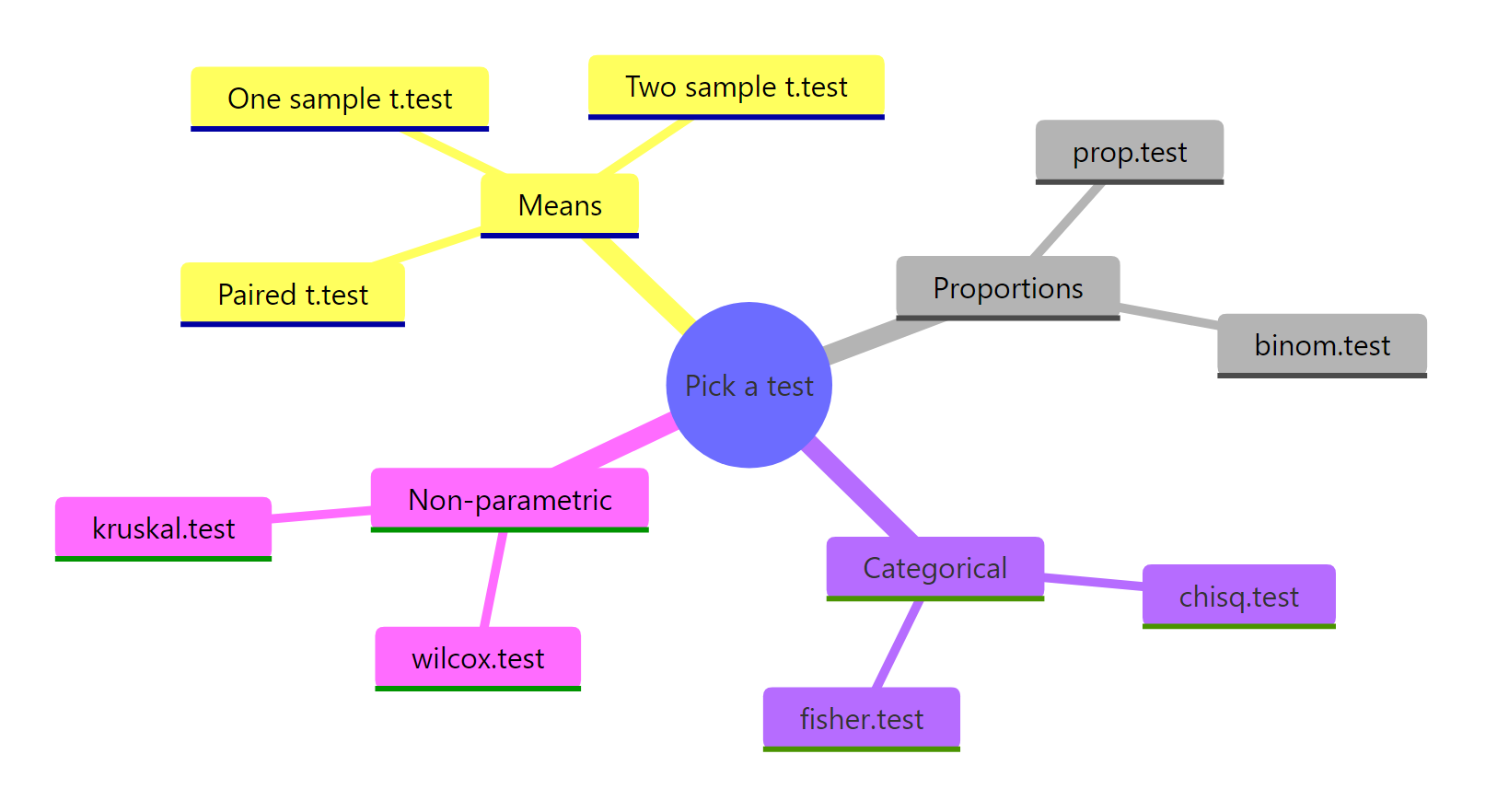
R's test families, organised by the data they accept.

Figure 3: R's test families, organised by the data they accept.

The hypothesis testing framework is the same five steps no matter which test you run. Once you have the steps internalised, switching from t.test() to prop.test() to chisq.test() is just changing one function call.

Step	What you do	R function / output field
1	State H₀ and H₁ before seeing data	(writing, your decision)
2	Choose the right test for your data shape	`t.test()`, `prop.test()`, `chisq.test()`, `wilcox.test()`
3	Compute the test statistic	`$statistic`
4	Compute the p-value	`$p.value`
5	Decide vs α, then report stat, df, p, CI, effect	compare to α; write up using all four

The single most important takeaway: a p-value is P(data this extreme | H₀ true), never the probability that H₀ is true. Internalise that and you'll stop misreading results, and you'll start asking for the confidence interval and effect size that p-values can never give you.

References

R Core Team, An Introduction to R. CRAN. Link
Wickham, H. & Grolemund, G., R for Data Science, 2nd Edition. Link
Wasserstein, R.L. & Lazar, N.A., The ASA's Statement on p-Values: Context, Process, and Purpose. The American Statistician, 70(2), 129-133 (2016). Link
Greenland, S. et al., Statistical tests, P values, confidence intervals, and power: a guide to misinterpretations. European Journal of Epidemiology, 31, 337-350 (2016). Link
R documentation, ?t.test, ?prop.test, ?chisq.test, ?wilcox.test. Run any of these at the R console for the canonical reference.
Cohen, J., Statistical Power Analysis for the Behavioral Sciences, 2nd Edition. Routledge (1988).
Dalpiaz, D., Applied Statistics with R. Link

Continue Learning

Confidence Intervals in R, the partner concept to hypothesis testing. Same data, different question: instead of "reject or not?" you ask "what range of values is plausible?" Most modern statisticians prefer reporting CIs alongside p-values.
Effect Size in R (Cohen's d, η², r), the "how big is it?" number that p-values cannot give you. Required for meta-analysis and any honest write-up.
Power Analysis in R, calculate the sample size you need before you collect data. Stops you running underpowered studies that fail to detect real effects.

Hypothesis Testing in R: Understand the Framework, Not Just the p-Value

What is the hypothesis testing framework?

How do you state the null and alternative hypothesis?

What is a test statistic and why does it matter?

What does the p-value really mean (and what doesn't it)?

How do you make a decision and avoid Type I and Type II errors?

How do you choose the right test for your data?

Practice Exercises

Exercise 1: One-sided t-test with a stricter α

Exercise 2: Empirical power across sample sizes

Complete Example: A Full Hypothesis Test, Reported Properly

Summary

References

Continue Learning

Further Reading

Related Tutorials