Chi-Square Goodness-of-Fit Test in R: Does Your Data Fit a Distribution?

The chi-square goodness-of-fit test in R checks whether observed category counts match an expected distribution. You hand chisq.test() your counts and the probabilities you expect, and it returns a single p-value telling you how surprised you should be by the data you saw.

What does the chi-square goodness-of-fit test actually answer?

Suppose you roll a die 60 times. A fair die should land on each face about 10 times. If face 5 came up 14 times and face 2 only 5 times, is the die loaded, or is that just luck? The chi-square goodness-of-fit test answers exactly this question. Pass chisq.test() your counts, and it scores how far the observed counts stray from the uniform distribution you'd expect.

RTest if a die is fair

# 60 rolls of a die, counts for faces 1 through 6 dice_obs <- c(8, 5, 9, 12, 14, 12) chisq.test(dice_obs) #> #> Chi-squared test for given probabilities #> #> data: dice_obs #> X-squared = 5.6, df = 5, p-value = 0.3471

The chi-square statistic is 5.6 across 5 degrees of freedom, and the p-value is 0.35. Because the p-value is well above 0.05, you do not reject the null hypothesis that the die is fair. In plain language: the wobble between counts is the kind you'd see by chance from a fair die roughly one time in three. By default, chisq.test() assumes a uniform distribution, which is why you didn't have to tell it what "fair" means. We'll override that default in the next section.

Try it: You flip a coin 100 times and record 58 heads and 42 tails. Use chisq.test() to test whether the coin is fair. Save the result to ex_coin_test.

RYour turn: test coin fairness

# Try it: test if a coin is fair after 100 flips ex_coin_obs <- c(58, 42) # Run chisq.test on ex_coin_obs and save to ex_coin_test ex_coin_test <- # your code here ex_coin_test #> Expected: X-squared = 2.56, df = 1, p-value ~ 0.11

Click to reveal solution

RCoin fairness solution

ex_coin_obs <- c(58, 42) ex_coin_test <- chisq.test(ex_coin_obs) ex_coin_test #> #> Chi-squared test for given probabilities #> #> data: ex_coin_obs #> X-squared = 2.56, df = 1, p-value = 0.1096

Explanation: With only two categories, the default uniform expectation is 50/50. A 58/42 split produces X-squared = 2.56 and p = 0.11, so you can't reject fairness at any standard threshold.

How do you test against custom probabilities?

Real distributions are rarely uniform. Mendel's classic dihybrid pea cross predicts a 9:3:3:1 ratio of yellow-round, yellow-wrinkled, green-round, and green-wrinkled peas. To check whether a sample matches that ratio, you pass the expected probabilities through the p = argument. Mendel's actual 1865 counts for those four categories were 315, 108, 101, and 32. Let's see how close they came.

RTest Mendel's 9:3:3:1 pea ratio

# Mendel's observed dihybrid cross counts peas_obs <- c(315, 108, 101, 32) # 9:3:3:1 ratio expressed as probabilities peas_exp <- c(9, 3, 3, 1) / 16 peas_exp #> [1] 0.5625 0.1875 0.1875 0.0625 peas_test <- chisq.test(peas_obs, p = peas_exp) peas_test #> #> Chi-squared test for given probabilities #> #> data: peas_obs #> X-squared = 0.47, df = 3, p-value = 0.9254

The p-value of 0.93 is enormous. The observed counts are almost suspiciously close to Mendel's prediction. You can keep the same peas_test object around for the rest of this post, since we'll mine it for residuals and effect size later. Notice that peas_exp had to sum to 1, which is why we divided the 9, 3, 3, 1 weights by 16. R will throw an error if your probabilities don't sum to 1.

Tip

Always pass probabilities, never raw ratios. chisq.test() requires p to sum to 1. If you have ratios like 9:3:3:1, divide by their total before passing to p, or set rescale.p = TRUE to let R do it for you.

Try it: Your marketing team expects website traffic to split 40% organic, 30% paid, 20% social, and 10% email. Last month you saw 412, 285, 220, and 83 visits in those channels. Test whether the actual mix matches the expected mix.

RYour turn: test marketing channel mix

# Try it: marketing channel goodness-of-fit ex_channels_obs <- c(412, 285, 220, 83) ex_channels_p <- c(0.40, 0.30, 0.20, 0.10) ex_channels_test <- # your code here ex_channels_test #> Expected: X-squared ~ 0.94, df = 3, p-value ~ 0.82

Click to reveal solution

RMarketing channel solution

ex_channels_obs <- c(412, 285, 220, 83) ex_channels_p <- c(0.40, 0.30, 0.20, 0.10) ex_channels_test <- chisq.test(ex_channels_obs, p = ex_channels_p) ex_channels_test #> #> Chi-squared test for given probabilities #> #> data: ex_channels_obs #> X-squared = 0.9433, df = 3, p-value = 0.8149

Explanation: A p-value of 0.81 means the observed mix is statistically indistinguishable from the planned mix. The campaign is hitting its targets.

How does R compute the chi-square statistic?

The function reports a number, but where does it come from? Walking through the math by hand makes the output stop feeling like magic. The recipe is simple: for each category, compute how far the observed count strays from the expected count, square it, divide by the expected count, then sum across categories.

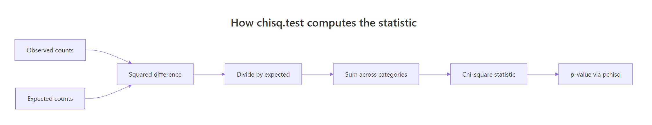
How the chi-square statistic is built from observed and expected counts.

Figure 1: How the chi-square statistic is built from observed and expected counts.

The intuition is that big categories naturally show bigger absolute deviations, so we scale the squared gap by what was expected. That keeps the contribution of each category fair regardless of size. Here is the formula:

$$\chi^2 = \sum_{i=1}^{k} \frac{(O_i - E_i)^2}{E_i}$$

Where:

$\chi^2$ = the chi-square statistic
$k$ = the number of categories
$O_i$ = the observed count in category $i$
$E_i$ = the expected count in category $i$ ($E_i = N \cdot p_i$, where $N$ is the total sample size)

The degrees of freedom are $k - 1$ for a goodness-of-fit test. The p-value is the area under a chi-square distribution with $k - 1$ degrees of freedom that lies to the right of the observed statistic. Now let's reproduce R's result by hand for the peas data.

RCompute chi-square by hand

# Expected counts: total sample size times each expected probability N <- sum(peas_obs) expected_counts <- peas_exp * N expected_counts #> [1] 312.75 104.25 104.25 34.75 # Sum of (O - E)^2 / E across categories chi_sq <- sum((peas_obs - expected_counts)^2 / expected_counts) chi_sq #> [1] 0.470024 # p-value is the upper tail of chi-square with k-1 df df_peas <- length(peas_obs) - 1 p_val <- 1 - pchisq(chi_sq, df = df_peas) p_val #> [1] 0.9254259

The hand-computed values match chisq.test() exactly. The expected counts (312.75, 104.25, 104.25, 34.75) are nearly identical to Mendel's observed counts (315, 108, 101, 32), so each squared deviation is small and the sum stays near zero. The function pchisq() returns the cumulative probability up to a value, so 1 - pchisq() gives the right tail, which is the p-value for goodness-of-fit.

Key Insight

The chi-square statistic is a weighted sum of surprises. Each category contributes a "surprise" equal to how far observed strayed from expected, squared so signs don't cancel, divided by what was expected so big categories don't dominate. A large total surprise across all categories is what produces a small p-value.

Try it: A factory expects 50% pass, 35% rework, and 15% scrap on its line. In a sample of 200 parts you observe 95 pass, 75 rework, and 30 scrap. Compute the chi-square statistic by hand and compare to chisq.test().

RYour turn: chi-square by hand

# Try it: factory QC ex_qc_obs <- c(95, 75, 30) ex_qc_p <- c(0.50, 0.35, 0.15) # Compute expected counts, the chi-square sum, and the p-value ex_qc_chi_sq <- # your code here ex_qc_chi_sq #> Expected: ~ 1.07

Click to reveal solution

RFactory QC solution

ex_qc_obs <- c(95, 75, 30) ex_qc_p <- c(0.50, 0.35, 0.15) ex_qc_N <- sum(ex_qc_obs) ex_qc_E <- ex_qc_p * ex_qc_N ex_qc_chi_sq <- sum((ex_qc_obs - ex_qc_E)^2 / ex_qc_E) ex_qc_chi_sq #> [1] 1.071429 # Verify with chisq.test chisq.test(ex_qc_obs, p = ex_qc_p)$statistic #> X-squared #> 1.071429

Explanation: Both the manual sum and chisq.test() produce X-squared = 1.07. They have to, because R is doing the same arithmetic.

What assumptions must your data meet?

The chi-square test rests on three assumptions you should verify before trusting the p-value. First, observations must be independent: each die roll, customer, or pea pod is its own data point. Second, categories must be mutually exclusive and exhaustive: every observation falls into exactly one category. Third, expected counts must be at least 5 in every category. The third assumption is the one R will warn you about, because the chi-square distribution approximation breaks down when expected counts get small.

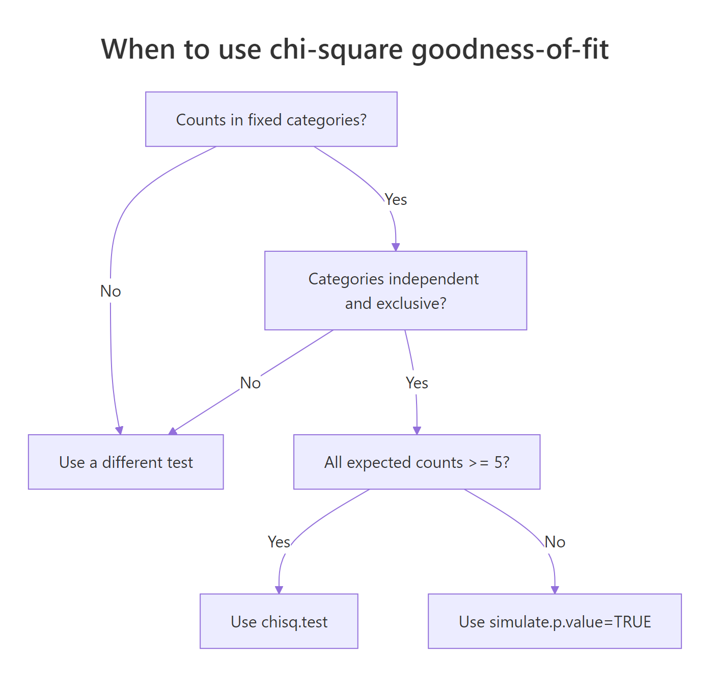
Decision flow: which form of the test to use based on expected counts.

Figure 2: Decision flow: which form of the test to use based on expected counts.

Let's deliberately trigger the small-N warning so you know what it looks like. The trick is to give chisq.test() a sample where one or more expected counts fall below 5.

RInspect expected counts and trigger the small-N warning

# Small sample: 15 observations across 5 categories, default uniform p small_obs <- c(2, 3, 4, 1, 5) small_test <- chisq.test(small_obs) #> Warning message: #> In chisq.test(small_obs) : Chi-squared approximation may be incorrect # Inspect the expected counts that triggered the warning small_test$expected #> [1] 3 3 3 3 3

Every expected count is 3, so all five categories violate the rule. R's warning is real, not cosmetic: with expected counts this small, the reported p-value can be off by a meaningful margin. The fix is to ask R to compute the p-value via Monte Carlo simulation rather than the chi-square approximation. The simulate.p.value = TRUE flag does exactly that, and B controls how many random tables to simulate.

RUse simulate.p.value when expected counts are below 5

# Monte Carlo p-value, robust to small expected counts small_mc <- chisq.test(small_obs, simulate.p.value = TRUE, B = 10000) small_mc #> #> Chi-squared test for given probabilities with simulated p-value #> (based on 10000 replicates) #> #> data: small_obs #> X-squared = 3.6667, df = NA, p-value = 0.4581

The Monte Carlo p-value is 0.46, which agrees with the asymptotic value here, but you don't get a "may be incorrect" warning. The trade-off is that the test no longer reports degrees of freedom (it shows df = NA) because Monte Carlo doesn't use the chi-square distribution.

Warning

Don't ignore the "approximation may be incorrect" warning. With small expected counts, the asymptotic p-value can be wrong by enough to flip your decision. Either pool sparse categories together, gather more data, or pass simulate.p.value = TRUE to switch to a Monte Carlo p-value.

Try it: A pet shop says 1 in 6 of its incoming kittens is black. In a small batch of 12 kittens, 5 are black. Use simulate.p.value = TRUE to test whether the shop's claim is consistent with this batch.

RYour turn: Monte Carlo for small samples

# Try it: pet shop kitten claim ex_kitten_obs <- c(5, 7) # black, not black ex_kitten_p <- c(1/6, 5/6) # Use simulate.p.value = TRUE to avoid the small-N warning ex_kitten_test <- # your code here ex_kitten_test #> Expected: X-squared ~ 7.2, p-value ~ 0.013

Click to reveal solution

RKitten claim solution

ex_kitten_obs <- c(5, 7) ex_kitten_p <- c(1/6, 5/6) set.seed(2026) ex_kitten_test <- chisq.test(ex_kitten_obs, p = ex_kitten_p, simulate.p.value = TRUE, B = 10000) ex_kitten_test #> #> Chi-squared test for given probabilities with simulated p-value #> (based on 10000 replicates) #> #> data: ex_kitten_obs #> X-squared = 7.2, df = NA, p-value = 0.0125

Explanation: Five black kittens in 12 is a lot more than the 2 you'd expect if 1 in 6 were black. The simulated p-value of about 0.013 says this is genuinely unusual, so the shop's claim looks shaky for this batch.

Which categories drive a significant result?

A small p-value tells you that something is off, but not where. To find the culprit categories, look at the standardized residuals. Each category gets a residual that behaves like a z-score: roughly normal with mean 0 and standard deviation 1 under the null. Values larger than about 2 in absolute size flag a category whose count surprised the test most.

RInspect Pearson and standardized residuals

# Pearson residuals: (O - E) / sqrt(E) peas_test$residuals #> [1] 0.12727922 0.36733378 -0.31866713 -0.46647416 # Standardized residuals: variance-corrected, comparable to z-scores peas_test$stdres #> [1] 0.39268272 0.59283832 -0.51422155 -0.55014836 # Combine into a tidy table for reporting res_table <- data.frame( category = c("Yellow Round", "Yellow Wrinkled", "Green Round", "Green Wrinkled"), observed = peas_obs, expected = round(peas_exp * sum(peas_obs), 2), pearson = round(peas_test$residuals, 3), stdres = round(peas_test$stdres, 3) ) res_table #> category observed expected pearson stdres #> 1 Yellow Round 315 312.75 0.127 0.393 #> 2 Yellow Wrinkled 108 104.25 0.367 0.593 #> 3 Green Round 101 104.25 -0.319 -0.514 #> 4 Green Wrinkled 32 34.75 -0.466 -0.550

Every standardized residual is well below 1 in absolute size, which lines up with the very high p-value. No single category is pulling on the test. For an even quicker read, plot the residuals against horizontal reference lines at +/-2.

RPlot standardized residuals with ggplot2

library(ggplot2) res_df <- data.frame( category = factor(res_table$category, levels = res_table$category), stdres = res_table$stdres ) ggplot(res_df, aes(x = category, y = stdres)) + geom_col(fill = "steelblue") + geom_hline(yintercept = c(-2, 2), linetype = "dashed", color = "red") + labs(title = "Standardized residuals: Mendel pea data", x = NULL, y = "Standardized residual") + theme_minimal()

All four bars are short and far inside the dashed reference lines. Visually that's the same story the table told: no category broke the test. When you see bars crossing the dashed lines, those categories are the ones to highlight in your write-up.

Note

Pearson residuals and standardized residuals are not the same thing. $residuals returns Pearson residuals: $(O - E) / \sqrt{E}$. $stdres returns standardized residuals, which divide further by an additional variance correction. The standardized version is what you compare to +/-2 because it actually behaves like a z-score under the null.

Try it: Customer arrivals across 5 weekdays were 18, 20, 24, 22, 36. Test uniformity, then identify which day has the most surprising count using standardized residuals.

RYour turn: weekday standardized residuals

# Try it: customer arrivals across weekdays ex_arr_obs <- c(18, 20, 24, 22, 36) # Run chisq.test, then identify the day with the largest |stdres| ex_arr_test <- # your code here ex_arr_stdres <- # your code here # Which weekday is the outlier? which.max(abs(ex_arr_stdres)) #> Expected: 5 (Friday, count 36 vs expected 24)

Click to reveal solution

RWeekday outlier solution

ex_arr_obs <- c(18, 20, 24, 22, 36) ex_arr_test <- chisq.test(ex_arr_obs) ex_arr_stdres <- ex_arr_test$stdres ex_arr_stdres #> [1] -1.5 -1.0 0.0 -0.5 3.0 which.max(abs(ex_arr_stdres)) #> [1] 5

Explanation: Friday's standardized residual is 3.0, well past +/-2, while every other day sits inside the band. The chi-square statistic is large because of Friday alone.

How big is the effect, not just the p-value?

Statistical significance and practical importance are different things. With a huge sample size, a tiny deviation can be highly significant. Effect size measures the size of the deviation in standardized units, independent of $N$. For chi-square, the standard effect size is Cohen's w. It is the square root of the chi-square statistic divided by the total sample size.

$$w = \sqrt{\frac{\chi^2}{N}}$$

Cohen's interpretation thresholds are 0.1 (small), 0.3 (medium), and 0.5 (large). Always report w alongside the p-value so readers can tell whether a "significant" finding is worth acting on.

RCompute Cohen's w effect size

# w = sqrt(chi-square / N) cohen_w <- sqrt(as.numeric(peas_test$statistic) / sum(peas_obs)) cohen_w #> [1] 0.02425354 # Interpret if (cohen_w < 0.1) cat("Effect size: negligible\n") #> Effect size: negligible

A w of 0.02 is well below "small" on Cohen's scale, confirming what the p-value already told us: Mendel's data fit the 9:3:3:1 prediction almost perfectly. In a study where you found a "significant" p-value of 0.04 on n = 100,000, a tiny w like 0.02 would let you tell stakeholders "yes it's significant, but the effect is not meaningful."

Tip

Always pair p-value and effect size in your report. A typical sentence reads: "The 9:3:3:1 ratio fits the data well (chi-square = 0.47, df = 3, p = 0.93, w = 0.02)." Reviewers and downstream readers can then judge importance, not just significance.

Try it: A test reports chi-square = 18.4 on a sample of N = 200. Compute Cohen's w and classify it.

RYour turn: classify effect size

# Try it: classify Cohen's w ex_chi <- 18.4 ex_n <- 200 ex_w <- # your code here ex_w #> Expected: ~ 0.303 (medium effect)

Click to reveal solution

REffect size classification solution

ex_chi <- 18.4 ex_n <- 200 ex_w <- sqrt(ex_chi / ex_n) ex_w #> [1] 0.3033150

Explanation: w = 0.30 sits right at Cohen's "medium" threshold. The deviation from the expected distribution is moderate, neither trivial nor large.

Practice Exercises

These capstone exercises combine multiple concepts from the tutorial. Use distinct variable names so they don't overwrite the tutorial state.

Exercise 1: Customer arrivals over a workweek

A coffee shop expects equal arrivals across Monday through Friday. Last week the counts were 42, 38, 51, 47, 92. Test uniformity, identify the surprising day from standardized residuals, and compute Cohen's w to judge effect size.

RCapstone 1: weekday arrivals

# Capstone 1: combine chisq.test, residuals, and effect size my_arrivals <- c(42, 38, 51, 47, 92) # Hint: chisq.test() with default p, then $stdres and Cohen's w my_arr_test <- # your code here # Which day is the outlier? # What is Cohen's w?

Click to reveal solution

RCapstone 1 solution

my_arrivals <- c(42, 38, 51, 47, 92) my_arr_test <- chisq.test(my_arrivals) my_arr_test #> #> Chi-squared test for given probabilities #> #> data: my_arrivals #> X-squared = 36.957, df = 4, p-value = 1.81e-07 # Standardized residuals my_arr_test$stdres #> [1] -1.207 -1.624 -0.083 -0.751 3.665 which.max(abs(my_arr_test$stdres)) #> [1] 5 # Effect size my_arr_w <- sqrt(as.numeric(my_arr_test$statistic) / sum(my_arrivals)) my_arr_w #> [1] 0.367

Explanation: The p-value is tiny, day 5 (Friday) has a standardized residual of 3.67 (well past +/-2), and Cohen's w of 0.37 is "medium-to-large." Friday is materially busier than the other days, so the manager should staff up.

Exercise 2: Birth months versus month-length probabilities

If birthdays were spread uniformly across the year, every month would get a share equal to its length divided by 365. In a sample of 600 people, the monthly counts (Jan to Dec) were 48, 41, 55, 49, 52, 47, 56, 51, 50, 53, 49, 49. Test the data against month-length probabilities and report the effect size.

RCapstone 2: birth months

# Capstone 2: custom probabilities + effect size my_births <- c(48, 41, 55, 49, 52, 47, 56, 51, 50, 53, 49, 49) my_month_p <- c(31, 28, 31, 30, 31, 30, 31, 31, 30, 31, 30, 31) / 365 # Hint: pass p = my_month_p to chisq.test, then compute Cohen's w my_birth_test <- # your code here my_birth_w <- # your code here

Click to reveal solution

RCapstone 2 solution

my_births <- c(48, 41, 55, 49, 52, 47, 56, 51, 50, 53, 49, 49) my_month_p <- c(31, 28, 31, 30, 31, 30, 31, 31, 30, 31, 30, 31) / 365 my_birth_test <- chisq.test(my_births, p = my_month_p) my_birth_test #> #> Chi-squared test for given probabilities #> #> data: my_births #> X-squared = 4.34, df = 11, p-value = 0.959 my_birth_w <- sqrt(as.numeric(my_birth_test$statistic) / sum(my_births)) my_birth_w #> [1] 0.085

Explanation: A p-value of 0.96 and w = 0.085 (below "small") means the observed births are perfectly consistent with month-length proportions. There is no birth-month clustering in this sample.

Putting It All Together

Let's run the full pipeline on a realistic example. A bag of M&M candies is supposed to follow Mars' published color ratio: 24% blue, 20% orange, 16% green, 14% yellow, 13% red, 13% brown. You count one bag and find 32 blue, 22 orange, 20 green, 18 yellow, 14 red, and 14 brown. Does this bag match the company's claim?

RM&M color distribution: end-to-end goodness-of-fit

library(ggplot2) # 1. Observed counts (one bag) and the published probabilities mm_obs <- c(blue = 32, orange = 22, green = 20, yellow = 18, red = 14, brown = 14) mm_exp <- c(blue = 0.24, orange = 0.20, green = 0.16, yellow = 0.14, red = 0.13, brown = 0.13) # 2. Run the test mm_test <- chisq.test(mm_obs, p = mm_exp) mm_test #> #> Chi-squared test for given probabilities #> #> data: mm_obs #> X-squared = 0.6927, df = 5, p-value = 0.9836 # 3. Assumption check: every expected count >= 5? mm_test$expected #> blue orange green yellow red brown #> 28.80 24.00 19.20 16.80 15.60 15.60 # All above 5, so the asymptotic p-value is trustworthy. # 4. Standardized residuals to see which colors deviate mm_test$stdres #> blue orange green yellow red brown #> 0.728 -0.456 0.222 0.319 -0.439 -0.439 # 5. Effect size mm_w <- sqrt(as.numeric(mm_test$statistic) / sum(mm_obs)) mm_w #> [1] 0.0759 # 6. Visualize residuals mm_res_df <- data.frame( color = factor(names(mm_obs), levels = names(mm_obs)), stdres = as.numeric(mm_test$stdres) ) ggplot(mm_res_df, aes(x = color, y = stdres, fill = color)) + geom_col() + geom_hline(yintercept = c(-2, 2), linetype = "dashed", color = "red") + scale_fill_manual(values = c(blue = "steelblue", orange = "orange", green = "forestgreen", yellow = "gold", red = "firebrick", brown = "saddlebrown")) + labs(title = "M&M standardized residuals vs. published ratio", x = NULL, y = "Standardized residual") + theme_minimal() + theme(legend.position = "none")

Conclusion you can write up: With X-squared = 0.69, df = 5, p = 0.98, w = 0.08, no expected count below 5, and every standardized residual well inside +/-2, the bag's color distribution is statistically indistinguishable from the company's published ratio.

Summary

The chi-square goodness-of-fit test reduces to four moves: get your counts, declare the expected probabilities, run chisq.test(), then probe the result for assumptions, residuals, and effect size.

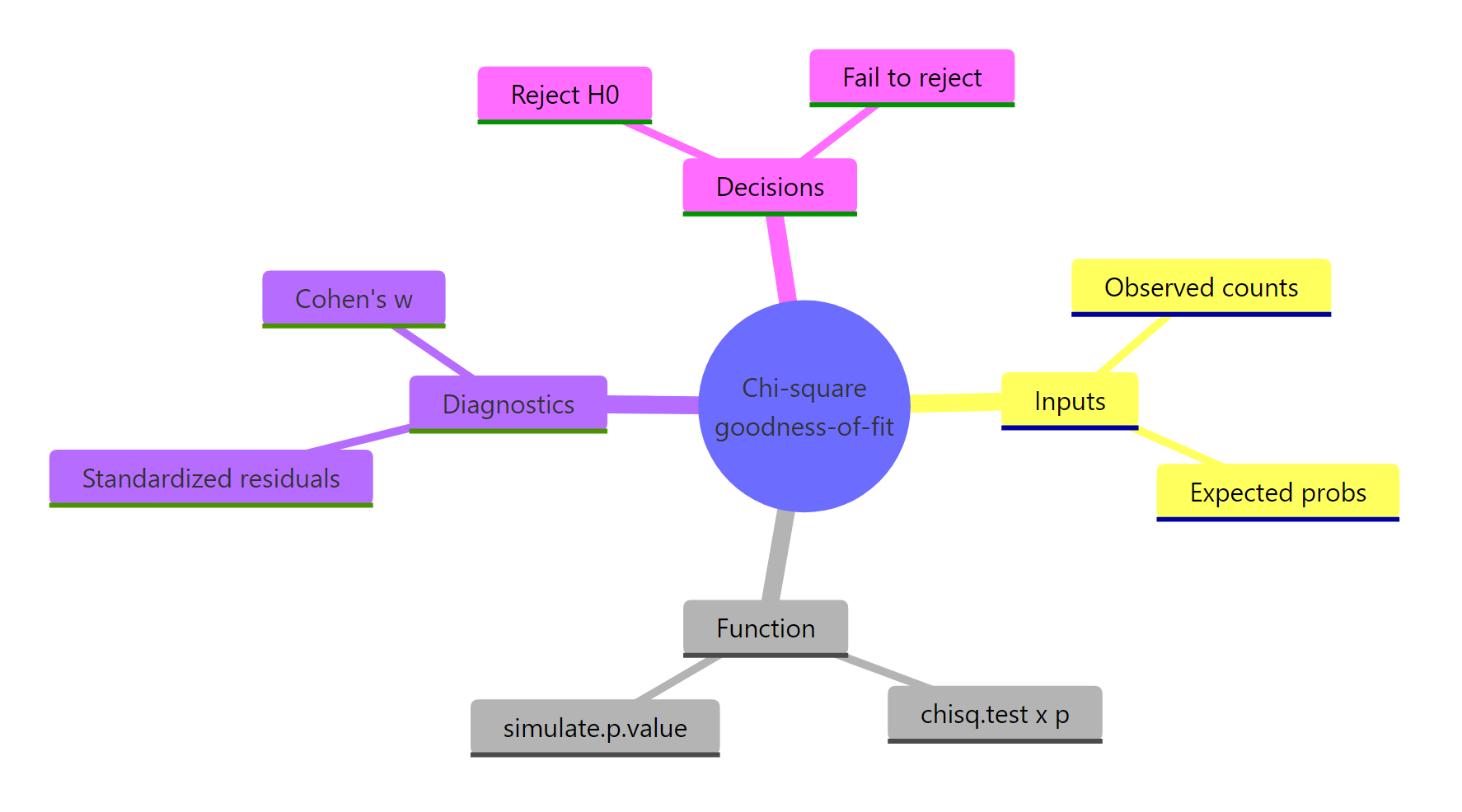
The four moving parts of a goodness-of-fit analysis at a glance.

Figure 3: The four moving parts of a goodness-of-fit analysis at a glance.

Step	Function or attribute	What it returns	When to use
Run the test	`chisq.test(x, p)`	Chi-square statistic, df, p-value	Every analysis
Check assumptions	`result$expected`	Expected counts per category	Before trusting the p-value
Handle small N	`simulate.p.value = TRUE`	Monte Carlo p-value	When any expected count < 5
Find the culprit	`result$stdres`	Z-like residual per category	After a small p-value
Quantify effect	`sqrt(chi-square / N)`	Cohen's w	Always, alongside the p-value
Visualize	`ggplot()` of residuals	Bar chart with +/-2 reference	Communicating findings

References

R Core Team. chisq.test, base R documentation. Link
Agresti, A. Categorical Data Analysis, 3rd Edition. Wiley (2013).
Cohen, J. Statistical Power Analysis for the Behavioral Sciences, 2nd Edition. Routledge (1988). Chapter 7 covers Cohen's w.
Sharpe, D. "Chi-Square Test is Statistically Significant: Now What?". Practical Assessment, Research & Evaluation, 20(8) (2015). Link
NIST/SEMATECH. e-Handbook of Statistical Methods, Section 1.3.5.15: Chi-Square Goodness-of-Fit. Link
Mendel, G. "Versuche über Pflanzenhybriden" (1865), translated as "Experiments in Plant Hybridization."
Wickham, H. & Grolemund, G. R for Data Science. Chapter on Exploratory Data Analysis. Link

Continue Learning

Chi-Square Test of Independence in R, the sister test for two-variable association in a contingency table.
Categorical Data in R, foundations of frequency tables and mosaic plots before you reach for chi-square.
Chi-Square Tests in R, a tour of the full chi-square family, including independence, homogeneity, and goodness-of-fit.

Chi-Square Goodness-of-Fit Test in R: Does Your Data Fit a Distribution?

What does the chi-square goodness-of-fit test actually answer?

How do you test against custom probabilities?

How does R compute the chi-square statistic?

What assumptions must your data meet?

Which categories drive a significant result?

How big is the effect, not just the p-value?

Practice Exercises

Exercise 1: Customer arrivals over a workweek

Exercise 2: Birth months versus month-length probabilities

Putting It All Together

Summary

References

Continue Learning

Related Tutorials