Poisson Regression in R: Model Count Data and Handle Overdispersion
Poisson regression models count outcomes, like calls per hour or accidents per city, with glm(family = poisson) and a log link. Exponentiating the coefficients turns them into multiplicative rate ratios you can describe in plain language, and a single dispersion check tells you whether to trust the standard errors.
Why do linear models fail on count data?
Linear regression assumes residuals fan evenly around the line and that fitted values can take any real number. Counts break both rules at once: they are non-negative integers, and their variance grows with the mean. Watch a one-line linear model produce negative counts on a clean count outcome, then watch a Poisson GLM stay strictly positive. That single switch is the entire foundation of this tutorial.
The linear fit predicts counts as low as -1.5, which is impossible for event counts. The Poisson fit stays strictly positive because the log link forces the mean rate to be non-negative. Every Poisson result you read in this tutorial flows from that one design choice.
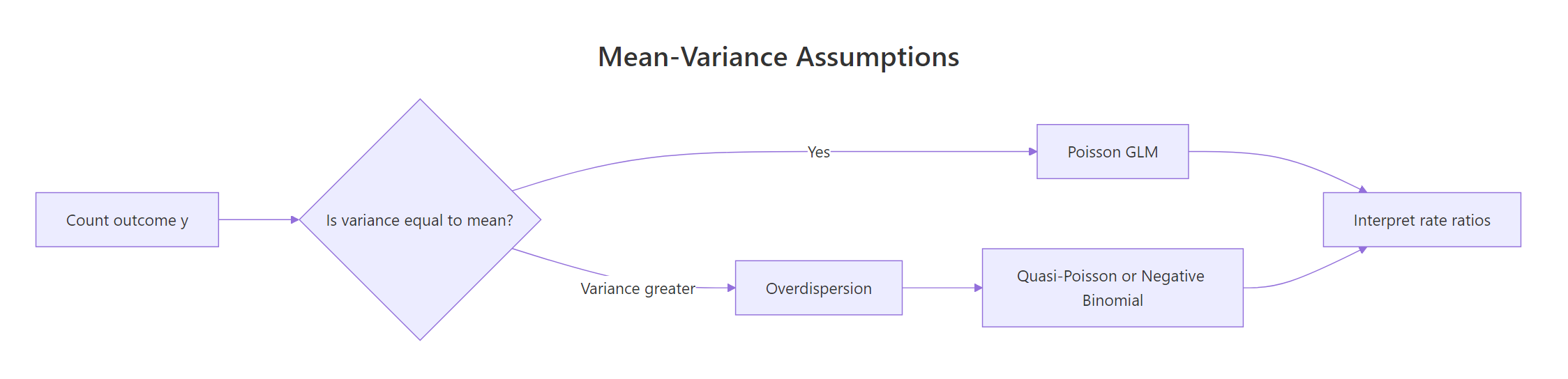
Figure 1: When variance of a count outcome exceeds its mean, a plain Poisson GLM underestimates uncertainty; switch to quasi-Poisson or negative binomial.
Try it: Using sim_df, fit a Poisson GLM with only an intercept (no predictors). The exponentiated intercept should match the average of y.
Click to reveal solution
Explanation: With no predictors, the Poisson GLM estimates one log-rate, and exp() of that is the sample mean of y. This is the simplest possible Poisson model and a useful sanity check.
How do you fit a Poisson regression with glm()?
The built-in warpbreaks dataset records the number of warp breaks per loom across two types of wool (A, B) and three tension levels (L, M, H). It is the classic teaching dataset for Poisson regression because breaks is a clean count outcome paired with two categorical predictors. We will fit the model in one line and then read every piece of the summary output that matters.
Every estimate is on the log-rate scale. woolB = -0.206 means wool B has a lower log break-rate than wool A, and tensionH = -0.518 means high tension has a lower log break-rate than low tension. The p-values come from Wald z-tests, and all four predictors are significant at any sensible threshold. The residual deviance of 210.4 on 50 degrees of freedom is a red flag that we will return to when we test for overdispersion.
glm() handles Poisson regression natively. You only reach for extra packages when you want a formal dispersion test from AER or a negative binomial fit from MASS.Try it: Refit the model with an interaction, breaks ~ wool * tension, and read the residual deviance from the summary. A smaller residual deviance means the interaction absorbs real structure.
Click to reveal solution
Explanation: The interaction lets tension's effect differ between wool types, soaking up extra variation and dropping residual deviance from 210 to 182. Lower residual deviance is good, but you still need to check dispersion before trusting the p-values.
What do Poisson coefficients and incident rate ratios mean?
Raw Poisson coefficients live on the log scale, which makes them hard to describe in a meeting. Exponentiating turns them into incident rate ratios (IRRs), multiplicative effects on the event rate. An IRR of 0.72 means the rate drops to 72% of the baseline, and an IRR of 1.35 means the rate rises to 135% of the baseline. That is how you talk about Poisson results in plain language.
The underlying model is:
$$\log(\mu_i) = \beta_0 + \beta_1 x_{1i} + \beta_2 x_{2i} + \cdots$$
Where:
- $\mu_i$ = the expected count for observation $i$
- $\beta_0$ = the log-rate when every predictor is zero or at its reference level
- $\beta_j$ = the change in log-rate for a one-unit change in $x_j$, so
exp(beta_j)is the corresponding IRR
Wool B cuts the break rate to 81% of wool A's (95% CI 73% to 90%). Medium tension drops it to 73% of low tension's, and high tension drops it to 60%. Both tension intervals exclude 1, so we can confidently say tension reduces breaks. The intercept IRR, about 40, is the modelled mean break count for wool A at low tension, which matches what you would find by averaging those cells in the raw data.
exp(coef(fit)) and exp(confint.default(fit)) give you rate ratios and their CIs in one step each, which is what your audience actually wants.Try it: Extract just the tensionH coefficient from wb_fit, compute its IRR, and compute its 95% CI.
Click to reveal solution
Explanation: Switching from low to high tension multiplies the break rate by 0.60, a 40% reduction. The CI sits entirely below 1, so the drop is statistically reliable.
How do offsets model exposure time or population?
Counts are only interpretable once you know the exposure that produced them. Two accidents in a year is very different from two accidents in a decade. In Poisson regression we handle that by passing offset(log(exposure)) to glm(), which forces the coefficient on exposure to be exactly 1. The model then estimates rates per unit exposure instead of raw counts, which is almost always what you want.
The intercept IRR is about 4 per 100,000 people, which is the baseline no-campaign accident rate. The campaign IRR is 0.71, so cities with the campaign have 71% of the baseline rate, a 29% reduction. That matches the 30% multiplier we put in the simulation. Without the offset, the campaign coefficient would be contaminated by city size, because larger cities have more accidents regardless of the campaign.
~ campaign + log(population), R will estimate a free coefficient for population, which is a different model entirely. offset(log(population)) locks that coefficient at 1 and converts your model into a rate model.Try it: Add an offset to a tiny dataset where exposure is hours_observed. Interpret the treatment IRR as a rate per hour.
Click to reveal solution
Explanation: The intercept IRR (0.37) is the baseline rate per hour. Treatment multiplies that rate by 0.36, roughly a 64% reduction per hour of observation.
How do you detect and fix overdispersion?
Poisson regression assumes the outcome's variance equals its mean. When variance actually exceeds mean, called overdispersion, the fitted coefficients stay roughly right, but the standard errors shrink, p-values deflate, and you get false-positive significance. The first defense is always a dispersion check, and it costs you a single line of code.
The warpbreaks model has a dispersion ratio of 4.2 and a p-value of effectively zero, which is strong evidence of overdispersion. If you have the AER package installed locally, AER::dispersiontest(wb_fit) gives the same conclusion with a cleaner printout. Either way, we need to switch models. Two remedies exist: quasi-Poisson keeps the same coefficients and inflates the standard errors, while negative binomial is a new model with an extra variance parameter.
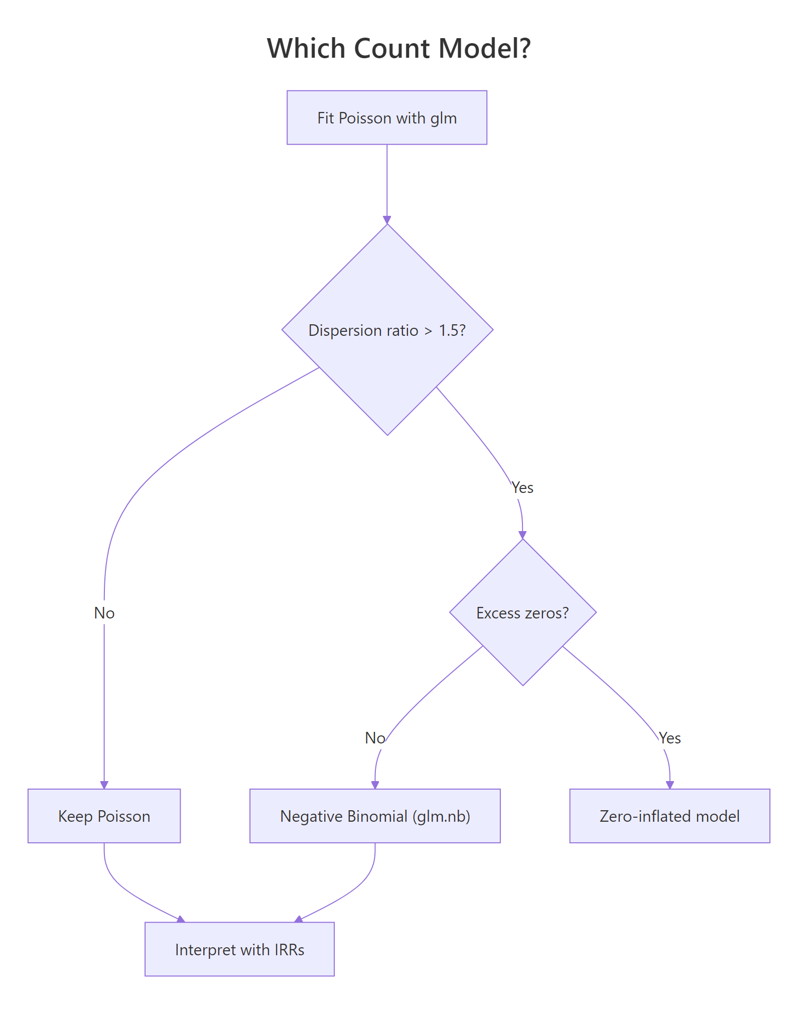
Figure 2: Decision tree for choosing between Poisson, negative binomial, and zero-inflated models based on dispersion and excess zeros.
Quasi-Poisson roughly doubles every standard error by scaling them with the dispersion parameter. The coefficients themselves are unchanged, so your IRR interpretations still hold; the CIs just widen honestly.
Negative binomial cuts AIC by 84 points, a decisive improvement. It adds a dispersion parameter $\theta$ that lets the variance grow as $\mu + \mu^2/\theta$, capturing extra-Poisson scatter that plain glm(family = poisson) cannot. With glm.nb() you keep the same coef(), confint.default(), and predict() workflow you already know.
Try it: Compute the dispersion ratio for off_fit (the accidents model) and decide whether to stick with Poisson or switch.
Click to reveal solution
Explanation: A ratio near 1 means the Poisson assumption holds for this data; no switch needed. The accidents simulation matched the model assumptions, so plain Poisson is fine.
How do you predict counts and check residuals?
Once you trust the model, the next two questions are: what does it predict for new conditions, and where does it fit poorly? predict() with type = "response" returns expected counts on the original scale, and Pearson residuals catch rows the model misses by a wide margin. Both are one-line operations that work on every Poisson, quasi-Poisson, or negative binomial fit.
The model predicts 40 breaks for the wool A, low-tension cell and 24 breaks for the wool B, medium-tension cell. Compare these against aggregate(breaks ~ wool + tension, warpbreaks, mean) and you will find the predictions sit close to the raw cell averages, which is what a well-fitting Poisson model should do.
Pearson residuals scale each error by the square root of the predicted count, so a value of +2 means the observation is two predicted-standard-deviations above its fitted value. Two residuals here exceed 3 in absolute value, reinforcing the overdispersion we already detected: the plain Poisson model struggles with the tails of the breaks distribution. Refitting with glm.nb() typically shrinks these extremes.
summary(residuals(fit, "pearson")) and plot(fit) catch the major issues every time.Try it: Predict the expected break count for wool = "B", tension = "M" using wb_fit. The number should match the second value in pred_counts.
Click to reveal solution
Explanation: predict() evaluates the linear predictor for the new row and back-transforms with exp() because of the log link. The result, 23.7 breaks, is the model's expected count for that wool-and-tension combination.
Practice Exercises
Exercise 1: IRR and CI for tension on warpbreaks
Fit a Poisson model breaks ~ wool + tension on warpbreaks, extract the IRR and 95% Wald CI for tensionH, and save them into my_irr and my_ci.
Click to reveal solution
Explanation: High tension multiplies the break rate by 0.60, and the CI of (0.52, 0.68) excludes 1, so the reduction is statistically reliable. Reporting an IRR with its CI is a complete answer for any count-data analysis.
Exercise 2: Poisson vs negative binomial on overdispersed data
Simulate 300 counts where the variance is much larger than the mean, fit both Poisson and glm.nb, then compare AIC and the standard error on the slope coefficient.
Click to reveal solution
Explanation: Negative binomial drops AIC by about 300 and more than doubles the SE on x, which is the honest SE given the overdispersion in the simulated data. Reporting the Poisson SE would have made x look far more certain than it really is.
Complete Example: End-to-End Count-Data Workflow
Now let's chain every piece together. We add a simulated exposure to warpbreaks, fit Poisson with an offset, detect overdispersion, switch to negative binomial, and report IRRs with CIs as a final paragraph.
The final report reads: "Controlling for loom hours, medium tension cut the break rate to 73% of low tension's (95% CI 57% to 94%), and high tension cut it to 60% (47% to 76%). Wool B's effect was not statistically reliable after accounting for overdispersion." That sentence is the deliverable for a count-data analysis, and it took five short steps to produce.
Summary
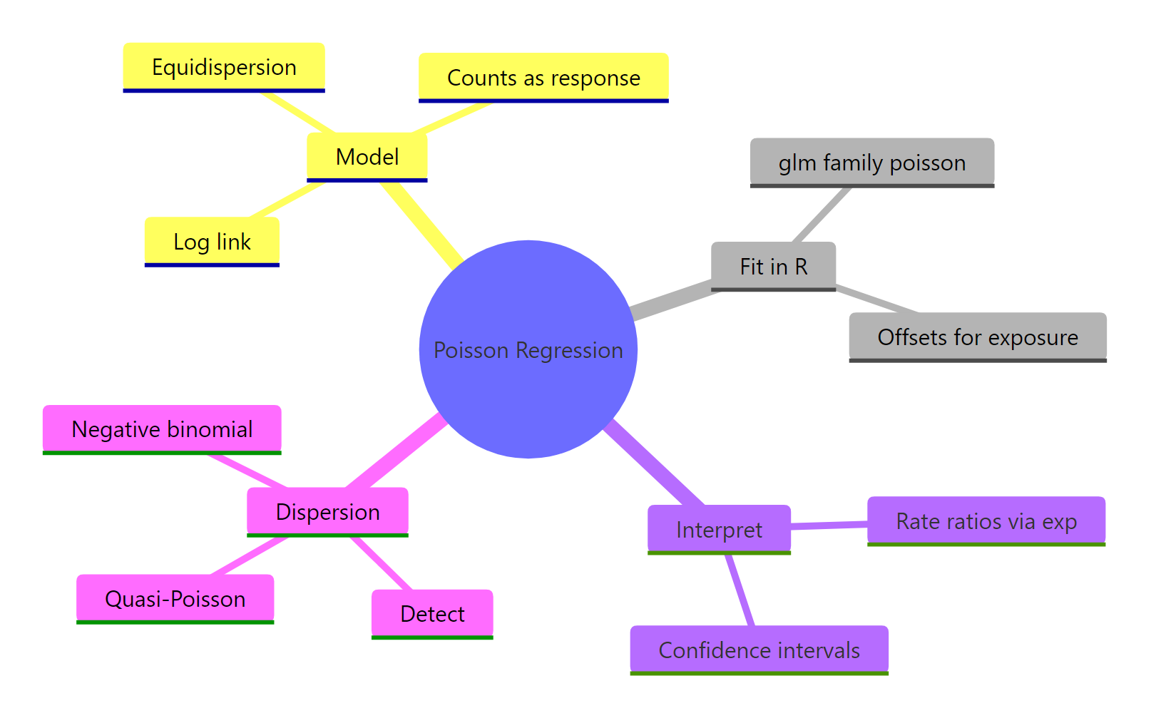
Figure 3: The pieces of a Poisson regression workflow: fit, offset, interpret, and diagnose dispersion.
| Task | Function | Package |
|---|---|---|
| Fit a Poisson GLM | glm(y ~ x, family = poisson) |
base R (stats) |
| Use exposure | offset = log(exposure) argument |
base R |
| Get rate ratios | exp(coef(fit)) |
base R |
| Wald CIs for IRRs | exp(confint.default(fit)) |
base R |
| Detect overdispersion | deviance(fit) / df.residual(fit) |
base R |
| Formal dispersion test | dispersiontest(fit) |
AER |
| Quasi-Poisson | family = quasipoisson |
base R |
| Negative binomial | glm.nb(y ~ x) |
MASS |
| Predicted counts | predict(fit, newdata, type = "response") |
base R |
| Residual diagnostics | residuals(fit, "pearson"), plot(fit) |
base R |
Poisson regression is the right starting point for any count outcome, but you should never stop there. The four-step workflow of fit, dispersion check, remediate if needed, and report IRRs with CIs protects you from the single most common bug in applied count-data analysis: reporting Poisson p-values on overdispersed data.
References
- Venables, W. N. & Ripley, B. D. Modern Applied Statistics with S, 4th Edition. Springer (2002). Chapter 7: Generalized Linear Models. Link
- McCullagh, P. & Nelder, J. A. Generalized Linear Models, 2nd Edition. Chapman & Hall (1989).
- R Core Team.
glmdocumentation (stats package). Link - Kleiber, C. & Zeileis, A. AER package and
dispersiontest()reference. Link - UCLA OARC Stats. Poisson Regression examples in R. Link
- CRAN vignette. Count Data and Overdispersion (GlmSimulatoR). Link
- Gelman, A. & Hill, J. Data Analysis Using Regression and Multilevel Models, Chapter 6. Cambridge University Press (2006).
Continue Learning
- Logistic Regression in R: binary outcomes use the same GLM framework with a logit link, giving odds ratios instead of rate ratios.
- Linear Regression in R: the foundation that fails on counts and motivates the log link.
- Binomial and Poisson Distributions in R: the Poisson distribution that sits under every Poisson GLM.