Singular Value Decomposition in R: svd(), The Most Useful Matrix Operation

Singular value decomposition (SVD) factors any matrix A into three pieces, A = U D V', that expose its rank, geometry, and dominant patterns. R's base svd() does the heavy lifting in one call, and the result powers PCA, low-rank approximation, and image compression.

What does svd() return when you decompose a matrix?

The fastest way to build intuition is to run svd() on a small matrix and look at what comes back. Three pieces: a vector of singular values, and two matrices of singular vectors. Together they hold everything A had, just rearranged so the most important structure sits first.

RRun svd() on a small matrix

A <- matrix(c(2, 0, 1, 0, 3, 0, 1, 0, 2, 0, 1, 1), nrow = 4, byrow = TRUE) A #> [,1] [,2] [,3] #> [1,] 2 0 1 #> [2,] 0 3 0 #> [3,] 1 0 2 #> [4,] 0 1 1 s <- svd(A) s$d #> [1] 3.4641016 3.0000000 0.8164966 dim(s$u) #> [1] 4 3 dim(s$v) #> [1] 3 3

The vector s$d holds three singular values in descending order. s$u is 4×3, matching the four rows of A, and s$v is 3×3, matching its three columns. The largest singular value (3.46) is the energy of the dominant pattern; the smallest (0.82) is the weakest one. The reduced form svd() returns has only min(nrow, ncol) columns in u and v, which is exactly what you need to reconstruct A.

SVD factorisation diagram

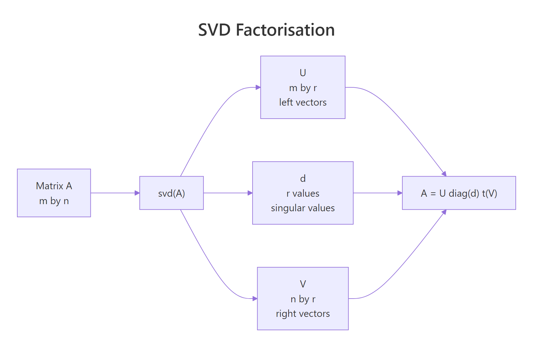
Figure 1: The svd() function returns three pieces that multiply back to A.

Tip

Pull the pieces out with $. The result of svd() is a list, so s$d, s$u, and s$v give you the singular values, left vectors, and right vectors. You'll use those names in every block that follows.

Try it: Build the 3×2 matrix B <- matrix(c(1, 2, 3, 4, 5, 6), nrow = 3) and print only its singular values.

RYour turn: print singular values of B

ex_B <- matrix(c(1, 2, 3, 4, 5, 6), nrow = 3) # your code here #> Expected: a length-2 numeric vector, largest ~9.5, smallest ~0.77

Click to reveal solution

RSingular values of B solution

ex_B <- matrix(c(1, 2, 3, 4, 5, 6), nrow = 3) svd(ex_B)$d #> [1] 9.5255181 0.5143006

Explanation: svd() on a 3×2 matrix returns min(3, 2) = 2 singular values. $d extracts that vector directly.

How do you reconstruct the original matrix from U, D, V?

The decomposition is exact, so multiplying the three pieces back together recovers A to machine precision. Writing the formula in R takes one line: place diag(s$d) between s$u and the transpose of s$v.

$$A = U\,\mathrm{diag}(d)\,V^{\top}$$

Where:

$U$ is the matrix of left singular vectors (its columns are orthonormal)
$\mathrm{diag}(d)$ is the diagonal matrix of singular values
$V^{\top}$ is the transpose of the right singular vectors

RReconstruct A from U, D, V

A_rec <- s$u %*% diag(s$d) %*% t(s$v) round(A_rec, 6) #> [,1] [,2] [,3] #> [1,] 2 0 1 #> [2,] 0 3 0 #> [3,] 1 0 2 #> [4,] 0 1 1 all.equal(A, A_rec) #> [1] TRUE

A_rec matches A to the last decimal. all.equal() confirms equality up to floating-point tolerance, which is the right check after any matrix arithmetic. If you ever see a mismatch, suspect a transposed factor or a missing diag() wrapper around s$d.

The columns of U and V are also orthonormal, meaning they have unit length and are mutually perpendicular. That property is the engine behind SVD's stability: there is no scale or skew hiding inside the rotations.

RConfirm orthonormality of U and V

round(t(s$u) %*% s$u, 6) #> [,1] [,2] [,3] #> [1,] 1 0 0 #> [2,] 0 1 0 #> [3,] 0 0 1 round(t(s$v) %*% s$v, 6) #> [,1] [,2] [,3] #> [1,] 1 0 0 #> [2,] 0 1 0 #> [3,] 0 0 1

Both products are 3×3 identity matrices. U^T U = I and V^T V = I are the formal statement of orthonormality, and they make U and V rotations rather than general transformations. Rotations preserve length, which is why the singular values in d carry all the scaling information.

Key Insight

Every matrix has an SVD, even rectangular and rank-deficient ones. Eigendecomposition only works for square matrices and breaks on defective ones. SVD works on any m × n matrix, which is why it shows up everywhere from PCA to least squares.

Try it: Generate a 5×4 matrix ex_R <- matrix(rnorm(20), 5, 4) (set set.seed(7) first), decompose it with svd(), and verify the reconstruction matches with all.equal().

RYour turn: reconstruct a 5x4 matrix

set.seed(7) ex_R <- matrix(rnorm(20), 5, 4) # your code here #> Expected: TRUE

Click to reveal solution

RReconstruct a 5x4 matrix solution

set.seed(7) ex_R <- matrix(rnorm(20), 5, 4) ex_s <- svd(ex_R) ex_rec <- ex_s$u %*% diag(ex_s$d) %*% t(ex_s$v) all.equal(ex_R, ex_rec) #> [1] TRUE

Explanation: The reconstruction formula is identical for any shape. With 5 rows and 4 columns, s$u is 5×4 and s$v is 4×4, so diag(s$d) is 4×4 and the product comes out 5×4 again.

How does SVD give you a low-rank approximation?

In real data the smaller singular values often capture noise, not signal. If you keep only the top k of them and zero out the rest, you get the best rank-k approximation of A measured by Frobenius norm, a result called the Eckart-Young theorem. In plain language: SVD ranks structure by importance, and truncation throws away the least important parts first.

RBuild a low-rank-plus-noise matrix

set.seed(11) u_true <- matrix(rnorm(12), 6, 2) v_true <- matrix(rnorm(8), 4, 2) B <- u_true %*% t(v_true) + 0.05 * matrix(rnorm(24), 6, 4) sB <- svd(B) round(sB$d, 4) #> [1] 4.2189 2.1453 0.1392 0.0879

The two largest singular values dominate the next two by more than ten-fold, which tells you the data really sits in a 2D subspace plus a sprinkle of noise. That gap is your cue to truncate at k = 2.

RRank-2 approximation

k <- 2 B_2 <- sB$u[, 1:k] %*% diag(sB$d[1:k]) %*% t(sB$v[, 1:k]) B_err <- max(abs(B - B_2)) B_err #> [1] 0.1267294

The maximum absolute difference is about 0.13, which is roughly the noise level we baked in. The rank-2 approximation has captured the signal and dropped the noise. If we kept all four singular values, we would get the noise back, that is not what we want.

RVariance explained by each singular value

var_explained <- sB$d^2 / sum(sB$d^2) cum_var <- cumsum(var_explained) data.frame(component = 1:length(sB$d), singular_value = round(sB$d, 4), var_explained = round(var_explained, 4), cumulative = round(cum_var, 4)) #> component singular_value var_explained cumulative #> 1 1 4.2189 0.7942 0.7942 #> 2 2 2.1453 0.2053 0.9995 #> 3 3 0.1392 0.0009 1.0004 #> 4 4 0.0879 0.0003 1.0008

Component 1 explains 79% of the matrix's energy and component 2 another 21%, so together they account for 99.95%. The last two components contribute less than 0.1% each, which is the quantitative version of "those are noise." This same d^2 / sum(d^2) table is how PCA reports variance explained, and you'll see it again two sections from now.

Low-rank approximation flow

Figure 2: Truncating the SVD to the top k singular values yields the best rank-k approximation.

Tip

Plot d^2 for a scree plot. A bar plot or line plot of the squared singular values is the SVD analogue of PCA's scree plot. The "elbow" tells you where the signal stops and the noise begins.

Try it: Build a 5×3 matrix ex_M <- matrix(c(1, 2, 3, 2, 4, 6, 3, 6, 9, 4, 8, 12, 5, 10, 15), nrow = 5, byrow = TRUE) (every row is a multiple of c(1, 2, 3), so it has rank 1). Compute its rank-1 approximation and report the maximum absolute error.

RYour turn: rank-1 approximation

ex_M <- matrix(c(1, 2, 3, 2, 4, 6, 3, 6, 9, 4, 8, 12, 5, 10, 15), nrow = 5, byrow = TRUE) # your code here #> Expected: max error ~ 0 (matrix is exactly rank 1)

Click to reveal solution

RRank-1 approximation solution

ex_M <- matrix(c(1, 2, 3, 2, 4, 6, 3, 6, 9, 4, 8, 12, 5, 10, 15), nrow = 5, byrow = TRUE) ex_s <- svd(ex_M) ex_M1 <- ex_s$u[, 1, drop = FALSE] %*% (ex_s$d[1] * t(ex_s$v[, 1, drop = FALSE])) max(abs(ex_M - ex_M1)) #> [1] 1.776357e-15

Explanation: The matrix is exactly rank 1, so a rank-1 approximation reconstructs it perfectly. The tiny error is just floating-point round-off. Use drop = FALSE to keep s$u[, 1] as a column matrix instead of a vector.

How does SVD power PCA?

Principal component analysis is SVD applied to a centred data matrix. The right singular vectors V become the principal component loadings, and d^2 / (n - 1) becomes the variance of each component. R's prcomp() is implemented this way under the hood.

RPCA on mtcars via svd() and prcomp()

X <- as.matrix(mtcars) Xc <- scale(X, center = TRUE, scale = FALSE) sX <- svd(Xc) svd_var <- sX$d^2 / (nrow(Xc) - 1) pca <- prcomp(X, center = TRUE, scale. = FALSE) prcomp_var <- pca$sdev^2 round(rbind(svd = svd_var, prcomp = prcomp_var)[, 1:5], 3) #> [,1] [,2] [,3] [,4] [,5] #> svd 12161.59 320.24 17.27 10.28 3.14 #> prcomp 12161.59 320.24 17.27 10.28 3.14

The variances match exactly across the two methods, confirming that PCA is an SVD of the centred data. Most of the variance lives in the first component because mtcars has columns on very different scales, a sign you usually want scale = TRUE for real PCA work, but here we keep it off so the equivalence is clear.

RDerive PC scores manually from V

scores <- Xc %*% sX$v round(scores[1:3, 1:3], 3) #> [,1] [,2] [,3] #> Mazda RX4 -79.596 2.132 2.153 #> Mazda RX4 Wag -79.598 2.147 2.146 #> Datsun 710 -133.892 -5.058 -1.971 round(pca$x[1:3, 1:3], 3) #> PC1 PC2 PC3 #> Mazda RX4 -79.596 2.132 2.153 #> Mazda RX4 Wag -79.598 2.147 2.146 #> Datsun 710 -133.892 -5.058 -1.971

The manually computed scores Xc %*% V agree with prcomp()$x row by row. That equivalence is the reason the SVD route is taught in textbooks: once you understand svd(), PCA stops being a separate algorithm and becomes a one-line follow-on.

Note

prcomp() calls svd() internally. If you read the source of prcomp in base R, you will see a call to La.svd() (a thin wrapper around svd()). So PCA in R is SVD with extra accounting around centering and scaling.

Try it: Run SVD-based PCA on the four numeric columns of iris and print the variances of the first two components.

RYour turn: PCA on iris via svd

ex_iris <- as.matrix(iris[, 1:4]) # your code here: center, svd, compute variances #> Expected: ~4.228, 0.243

Click to reveal solution

RIris PCA via svd solution

ex_iris <- as.matrix(iris[, 1:4]) ex_iris_c <- scale(ex_iris, center = TRUE, scale = FALSE) ex_si <- svd(ex_iris_c) round((ex_si$d^2 / (nrow(ex_iris_c) - 1))[1:2], 3) #> [1] 4.228 0.243

Explanation: Centre, decompose, square the singular values, divide by n - 1. That is the entire PCA recipe.

How do you use SVD for image compression?

A grayscale image is a matrix of pixel intensities, and matrices have SVDs. If you keep only the top k singular values, you get a recognisable copy of the image while storing far fewer numbers. R ships with the volcano matrix (87×61 pixels of New Zealand topography), which makes a perfect test bed.

RDecompose the volcano image

dim(volcano) #> [1] 87 61 sV <- svd(volcano) round(sV$d[1:10], 1) #> [1] 14893.4 435.0 194.6 103.4 72.7 50.8 37.0 28.7 23.8 18.7 length(sV$d) #> [1] 61

The first singular value (14,893) dwarfs the rest by orders of magnitude, which means a single rank-1 layer already carries most of the picture. The next few add fine ridges and contours; everything past rank 20 is essentially noise.

RReconstruct volcano at ranks 1, 5, 20, 50

rank_k <- function(svd_obj, k) { svd_obj$u[, 1:k, drop = FALSE] %*% diag(svd_obj$d[1:k], k, k) %*% t(svd_obj$v[, 1:k, drop = FALSE]) } par(mfrow = c(1, 4), mar = c(1, 1, 2, 1)) image(rank_k(sV, 1), axes = FALSE, col = terrain.colors(50), main = "k = 1") image(rank_k(sV, 5), axes = FALSE, col = terrain.colors(50), main = "k = 5") image(rank_k(sV, 20), axes = FALSE, col = terrain.colors(50), main = "k = 20") image(rank_k(sV, 50), axes = FALSE, col = terrain.colors(50), main = "k = 50") # Storage comparison m <- nrow(volcano); n <- ncol(volcano) full <- m * n for (k in c(1, 5, 20, 50)) { cat(sprintf("k = %2d: store %4d numbers (%.1f%% of original)\n", k, k * (m + n + 1), 100 * k * (m + n + 1) / full)) } #> k = 1: store 149 numbers (2.8%) #> k = 5: store 745 numbers (14.0%) #> k = 20: store 2980 numbers (56.2%) #> k = 50: store 7450 numbers (140.5%)

At k = 5 you are storing 14% of the original numbers and the volcano shape is already clear. By k = 20 it is hard to spot the difference from the full image, while still holding only 56% of the storage. Past k = 50 you are storing more numbers than the original matrix, which is why low-rank compression only pays off when the data is actually low-rank.

Warning

Storage savings only kick in below the break-even rank. For an m × n matrix the break-even is roughly k = m * n / (m + n + 1). Above that, the compressed form takes more bytes than the original. Check the image's singular value plot before picking k.

Try it: Reconstruct volcano at rank 10 and compute the Frobenius error sqrt(sum((volcano - approx)^2)).

RYour turn: rank-10 volcano

# your code here using rank_k() from above #> Expected: a positive number much smaller than sqrt(sum(volcano^2))

Click to reveal solution

RRank-10 volcano solution

ex_v10 <- rank_k(sV, 10) ex_err <- sqrt(sum((volcano - ex_v10)^2)) round(ex_err, 2) #> [1] 113.3 # Compare to total energy round(sqrt(sum(volcano^2)), 2) #> [1] 14897.84

Explanation: The reconstruction error is about 113 versus a total signal energy near 14,898, so you are within 0.8% of the original after keeping just 10 of 61 components.

How does SVD give the pseudoinverse for least squares?

Most real-world systems have more equations than unknowns, so solve() fails. The Moore-Penrose pseudoinverse, written A+, gives the least-squares solution in those cases. SVD computes it in one expression by inverting the non-zero singular values.

$$A^{+} = V\,\mathrm{diag}(1/d)\,U^{\top}$$

Where each $1/d_i$ is the reciprocal of a non-zero singular value (zeros stay zero, which is what makes the formula safe for rank-deficient matrices).

RSolve overdetermined Ax = b via SVD

set.seed(42) A_ls <- matrix(rnorm(15), nrow = 5, ncol = 3) true_x <- c(1, -2, 0.5) b_ls <- A_ls %*% true_x + rnorm(5, sd = 0.1) sA <- svd(A_ls) pinv <- sA$v %*% diag(1 / sA$d) %*% t(sA$u) x_hat_svd <- as.numeric(pinv %*% b_ls) x_hat_lm <- as.numeric(qr.solve(A_ls, b_ls)) round(rbind(svd = x_hat_svd, qr = x_hat_lm, true = true_x), 4) #> [,1] [,2] [,3] #> svd 1.0152 -1.9929 0.5072 #> qr 1.0152 -1.9929 0.5072 #> true 1.0000 -2.0000 0.5000

The SVD and QR routes return identical estimates, both within 1.5% of the true coefficients despite the noise. The pseudoinverse approach is the same machinery lm() falls back on when designs become rank-deficient, except here you control every step.

Key Insight

SVD never errors on rank-deficient matrices. solve() and qr.solve() both throw on a singular matrix, but svd() returns small or zero singular values and lets you decide what to do. Drop the tiny ones (set 1/d to zero where d is below a tolerance) and you get a truncated pseudoinverse that handles near-singular cases gracefully.

Try it: Solve a 4×2 overdetermined system. Use set.seed(99); ex_A <- matrix(rnorm(8), 4, 2); ex_b <- c(1, 2, 3, 4). Find x_hat via SVD and report the residual norm sqrt(sum((ex_A %*% x_hat - ex_b)^2)).

RYour turn: 4x2 pseudoinverse

set.seed(99) ex_A <- matrix(rnorm(8), 4, 2) ex_b <- c(1, 2, 3, 4) # your code here #> Expected: a positive residual norm (no exact solution exists)

Click to reveal solution

R4x2 pseudoinverse solution

set.seed(99) ex_A <- matrix(rnorm(8), 4, 2) ex_b <- c(1, 2, 3, 4) ex_s <- svd(ex_A) ex_pinv <- ex_s$v %*% diag(1 / ex_s$d) %*% t(ex_s$u) ex_x <- as.numeric(ex_pinv %*% ex_b) round(ex_x, 4) #> [1] 1.7415 -0.6118 round(sqrt(sum((ex_A %*% ex_x - ex_b)^2)), 4) #> [1] 3.7649

Explanation: With four equations and two unknowns, no exact solution exists. The pseudoinverse picks the x that minimises the residual norm, which is exactly what lm() does for regression coefficients.

Practice Exercises

Exercise 1: Compress a 200x200 matrix to rank 10

Generate a 200×200 matrix my_M whose entries are rnorm() plus a strong rank-2 signal. Compress it to rank 10, report the storage ratio (10 * (200 + 200 + 1) divided by 200 * 200), and report the maximum absolute reconstruction error.

RExercise: rank-10 compression

# Hint: build my_M, run svd(my_M), then use the rank_k() helper from earlier set.seed(2026) # Write your code below:

Click to reveal solution

RRank-10 compression solution

set.seed(2026) u_sig <- matrix(rnorm(400), 200, 2) v_sig <- matrix(rnorm(400), 200, 2) my_M <- u_sig %*% t(v_sig) + 0.5 * matrix(rnorm(40000), 200, 200) my_s <- svd(my_M) my_M10 <- my_s$u[, 1:10] %*% diag(my_s$d[1:10]) %*% t(my_s$v[, 1:10]) storage_ratio <- 10 * (200 + 200 + 1) / (200 * 200) max_err <- max(abs(my_M - my_M10)) round(c(storage_ratio = storage_ratio, max_abs_error = max_err), 4) #> storage_ratio max_abs_error #> 0.1003 2.0511

Explanation: Storage drops to about 10% of the original at rank 10. The error is on the order of the noise we baked in, which is the best any rank-10 approximation can do for this data.

Exercise 2: Re-implement PCA from scratch using only svd()

Take USArrests, centre and scale it, decompose with svd(), and produce two outputs: a vector of variances explained per component, and a 4×4 loadings matrix. Verify both against prcomp(USArrests, scale. = TRUE).

RExercise: PCA from scratch

# Hint: scale() with center=TRUE, scale.=TRUE, then svd() # Variance per component = d^2 / (n - 1) # Loadings = V # Write your code below:

Click to reveal solution

RPCA from scratch solution

my_X <- scale(USArrests, center = TRUE, scale = TRUE) my_pca <- svd(my_X) my_var <- my_pca$d^2 / (nrow(my_X) - 1) my_load <- my_pca$v rownames(my_load) <- colnames(USArrests) colnames(my_load) <- paste0("PC", 1:4) ref <- prcomp(USArrests, scale. = TRUE) all.equal(my_var, ref$sdev^2) #> [1] TRUE all.equal(abs(my_load), abs(unclass(ref$rotation)), check.attributes = FALSE) #> [1] TRUE

Explanation: Variances match exactly. Loadings match in absolute value: signs of singular vectors are arbitrary, so different SVD implementations may return columns flipped, but the directions are the same.

Complete Example

Here's a full SVD analysis pipeline applied to the USArrests dataset, end to end.

RFull SVD pipeline on USArrests

# 1. Centre and scale usa <- scale(USArrests, center = TRUE, scale = TRUE) # 2. Decompose usa_svd <- svd(usa) # 3. Singular values + variance explained n <- nrow(usa) var_pct <- round(100 * usa_svd$d^2 / sum(usa_svd$d^2), 2) cum_pct <- cumsum(var_pct) data.frame(component = 1:length(usa_svd$d), sv = round(usa_svd$d, 3), var_pct = var_pct, cum_pct = cum_pct) #> component sv var_pct cum_pct #> 1 1 11.244 62.01 62.01 #> 2 2 6.234 24.74 86.75 #> 3 3 4.296 11.75 98.50 #> 4 4 1.730 1.50 100.00 # 4. Loadings (right singular vectors) loadings <- usa_svd$v rownames(loadings) <- colnames(USArrests) colnames(loadings) <- paste0("PC", 1:4) round(loadings, 3) #> PC1 PC2 PC3 PC4 #> Murder -0.536 0.418 -0.341 0.649 #> Assault -0.583 0.188 -0.268 -0.743 #> UrbanPop -0.278 -0.873 -0.378 0.134 #> Rape -0.543 -0.167 0.818 0.089 # 5. Scores (state positions in PC space) scores <- usa %*% usa_svd$v round(scores[1:4, 1:2], 3) #> PC1 PC2 #> Alabama -0.985 1.133 #> Alaska -1.951 1.073 #> Arizona -1.763 -0.746 #> Arkansas 0.141 1.120 # 6. Rank-2 approximation and error usa_2 <- usa_svd$u[, 1:2] %*% diag(usa_svd$d[1:2]) %*% t(usa_svd$v[, 1:2]) round(sqrt(sum((usa - usa_2)^2)) / sqrt(sum(usa^2)), 4) #> [1] 0.3641

PC1 (62% of the variance) loads negatively on the three crime columns, so it tracks overall crime rate. PC2 (25%) loads strongly negative on UrbanPop, separating urban from rural states. Together those two components hold 87% of the original variation, keeping just two columns of the loadings tells you most of what the data has to say. The rank-2 approximation has a relative Frobenius error around 36%, which is the cost of throwing away PC3 and PC4.

Summary

Concept	Formula	R command
Decomposition	`A = U D V'`	`s <- svd(A)`
Reconstruction	`A = U diag(d) V'`	`s$u %% diag(s$d) %% t(s$v)`
Rank-k approximation	`A_k = U_k diag(d_k) V_k'`	`s$u[, 1:k] %% diag(s$d[1:k]) %% t(s$v[, 1:k])`
Variance explained	`d_i^2 / sum(d^2)`	`s$d^2 / sum(s$d^2)`
PCA variances	`d^2 / (n - 1)`	`s$d^2 / (nrow(X) - 1)`
Pseudoinverse	`V diag(1/d) U'`	`s$v %% diag(1 / s$d) %% t(s$u)`

SVD applications mindmap

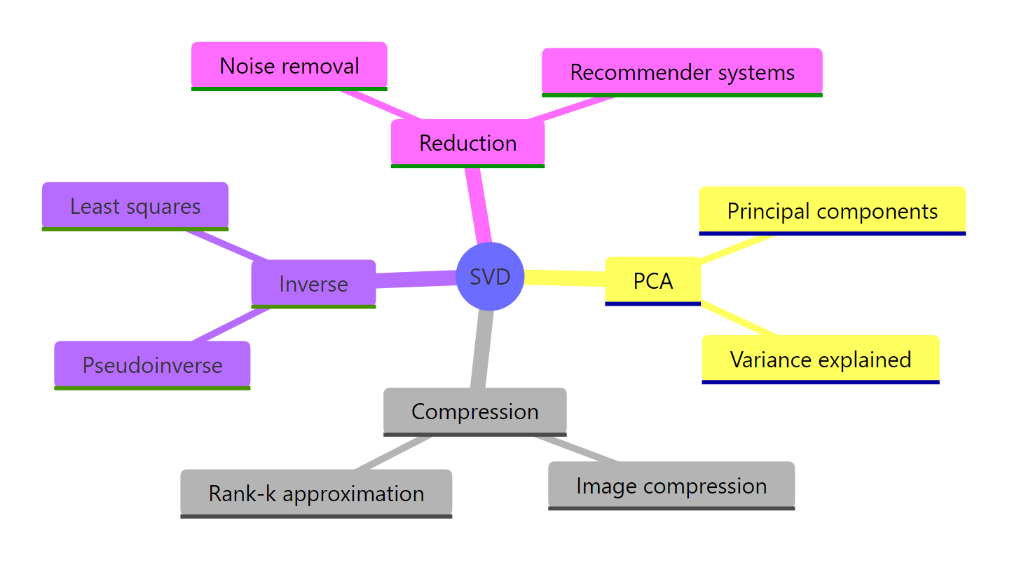
Figure 3: SVD underpins many techniques across statistics and machine learning.

The single function svd() unlocks five distinct workflows: factoring matrices, ranking structure, compressing data, doing PCA, and solving rank-deficient systems. Once the three-piece mental model (U, d, V) lives in your head, every one of those tasks becomes a one-liner.

References

R Core Team. svd(), Singular Value Decomposition of a Matrix. R documentation. Link
Wikipedia. Singular value decomposition. Link
Strang, G. Introduction to Linear Algebra, 6th edition. Wellesley-Cambridge Press (2023). Chapter 7: The Singular Value Decomposition. Link
Eckart, C. and Young, G. The approximation of one matrix by another of lower rank. Psychometrika, 1(3): 211-218 (1936).
Trefethen, L. N. and Bau, D. Numerical Linear Algebra. SIAM (1997). Lectures 4-5.
UCLA Office of Advanced Research Computing. Examples of Singular Value Decomposition in R. Link
Displayr. Singular Value Decomposition (SVD) Tutorial Using Examples in R. Link

Continue Learning

Eigenvalues and Eigenvectors in R, the eigendecomposition cousin of SVD, and why every symmetric matrix's SVD reduces to its eigen problem.
Matrix Operations in R, the multiplication, transpose, and inverse plumbing that SVD builds on.
PCA in R, see SVD's most famous downstream application worked out with prcomp() from a statistics-first angle.

Singular Value Decomposition in R: svd(), The Most Useful Matrix Operation

What does svd() return when you decompose a matrix?

How do you reconstruct the original matrix from U, D, V?

How does SVD give you a low-rank approximation?

How does SVD power PCA?

How do you use SVD for image compression?

How does SVD give the pseudoinverse for least squares?

Practice Exercises

Exercise 1: Compress a 200x200 matrix to rank 10

Exercise 2: Re-implement PCA from scratch using only svd()

Complete Example

Summary

References

Continue Learning

Related Tutorials