Bayesian Logistic Regression in R: Why Stakeholders Trust These Odds Ratios More
A frequentist glm(family = binomial) returns log-odds coefficients with a standard error and a p-value. Translating that to "the odds of conversion go up by 38%" requires careful interpretation of confidence intervals on a transformed scale. A Bayesian logistic regression returns a full posterior over the log-odds, which converts trivially to a posterior over odds ratios and probabilities. Stakeholders read "82% probability the odds ratio exceeds 1.5" much more easily than a p-value. This post fits a Bayesian logistic regression with brms end to end and walks through every output.
What does Bayesian logistic regression buy you over glm(family = binomial)?
glm() for binary outcomes returns a single estimate per coefficient on the log-odds scale, plus a standard error. To get an odds ratio you exponentiate the estimate; to get a probability for a specific scenario you push it through plogis(). Confidence intervals on the original scale do not translate cleanly to the transformed scale; you need the delta method or a profile likelihood.
A Bayesian logistic regression returns a full posterior over each coefficient. To get an odds ratio posterior, exponentiate every draw. To get a probability posterior at a specific x, push every draw through plogis(). Every quantity has a credible interval; every probability statement is trivial.
Walk through what just happened. We coded the binary outcome y_8cyl as 1 when the car has 8 cylinders. The brms call uses family = bernoulli("logit") to specify a logistic regression. Four chains and 2000 iterations is the standard.
The posterior summary gives log-odds coefficients. The mpg coefficient is -0.43 with 95% credible interval [-1.06, 0.14]. On the log-odds scale, this says one extra mpg multiplies the odds of being 8-cyl by exp(-0.43) = 0.65 (35% reduction).
The wt coefficient is 1.42 with credible interval [-1.02, 4.04]. The interval crosses zero, which means the data does not strongly identify the wt effect after accounting for mpg.
exp() (for odds ratios) or plogis() (for probabilities) before reporting to stakeholders. The next sections walk through both conversions on the posterior draws.Try it: Compute the posterior probability that the mpg coefficient is below -0.2 (a meaningful negative effect on the log-odds of being 8-cyl).
Click to reveal solution
About 79% posterior probability that one extra mpg reduces the log-odds of being 8-cyl by at least 0.2 (an odds ratio of exp(-0.2) = 0.82 or 18% reduction). That is a clean probability statement on a scale stakeholders care about.
How do I fit one in brms?
Two changes from the linear regression workflow: set family = bernoulli("logit") and use posterior_epred() (which returns probabilities on [0, 1]) instead of posterior_predict() (which returns 0/1 outcomes) when you want the probability of the event.
Walk through the priors. normal(0, 2.5) on the slopes is the Stan team's recommended default for log-odds slopes. Half of the prior's mass is between -1.7 and 1.7, which corresponds to odds ratios between 0.18 and 5.5, a wide but not absurd range. normal(0, 1.5) on the intercept centres at log-odds 0 (probability 0.5 at zero predictors) with reasonable spread.
Compare the priors-set fit to the default. The posterior mean for mpg shifted from -0.43 (default flat prior on slope) to -0.27 (with normal(0, 2.5)). The credible interval tightened from [-1.06, 0.14] to [-0.62, 0.02]. With 32 observations, the prior contributes meaningfully; the choice between flat and weakly informative is real.
The Rhat and Bulk_ESS values are clean. We can read the posterior with confidence.
exp(100) or larger. Use normal(0, 2.5) or normal(0, 1) as the default; tighten only if you have specific knowledge.Try it: Refit with prior(normal(0, 0.5), class = "b") and observe how the slope posterior tightens around zero.
Click to reveal solution
The tight prior pulled the mpg posterior mean from -0.27 to -0.21. The credible interval narrowed from [-0.62, 0.02] to [-0.51, 0.07]. The data still drives the sign and magnitude, but the prior contributed real shrinkage.
How do I read the log-odds posterior?
The posterior mean is on the log-odds scale: it tells you how much the log-odds of the event change per unit increase in the predictor. The credible interval is also on the log-odds scale.
Three things to look at:
The first is sign and significance. Does the credible interval exclude zero? If yes, the predictor's effect is reliable in the direction of the posterior mean. If the interval crosses zero, the data does not pin down the sign.
The second is magnitude. A log-odds coefficient of 0.5 corresponds to an odds ratio of exp(0.5) = 1.65 (65% increase in odds). A coefficient of -0.5 corresponds to exp(-0.5) = 0.61 (39% decrease in odds). Build intuition for the conversion.
The third is uncertainty. A coefficient of 0.5 with credible interval [0.4, 0.6] is a tight estimate. The same posterior mean with interval [-0.5, 1.5] is essentially nothing learned.
Walk through the conversion. Each row shows the log-odds estimate alongside its odds-ratio counterpart. For mpg, the estimate of -0.27 corresponds to an odds ratio of 0.76 (24% reduction in odds of being 8-cyl per extra mpg). The 95% credible interval on the odds-ratio scale is [0.54, 1.02].
Notice how wt looks different on the two scales. The log-odds estimate is 0.83 with interval [-0.62, 2.49]. On the odds-ratio scale, the same translates to 2.29 with interval [0.54, 12.06].
The right tail of the interval (12) is huge because exp() blows up at the top end of a wide interval. This is why direct log-odds intervals are sometimes more informative than odds-ratio intervals: the latter can be misleadingly large.
exp(0.5) = 1.65), an odds ratio (just 0.5, halved odds), or a probability (plogis(0.5) ≈ 0.62). Be explicit in your text and column headers.Try it: Compute the posterior median odds ratio for mpg and a 50% credible interval on it.
Click to reveal solution
Posterior median odds ratio for mpg is 0.77, with 50% credible interval [0.69, 0.85]. That means a 50% probability the odds of being 8-cyl multiply by between 0.69 and 0.85 per extra mpg.
How do I convert log-odds to odds ratios and probabilities?
Two conversions and one R idiom for each.
Log-odds to odds ratio: exp(coef). exp(0.5) = 1.65 says the odds multiply by 1.65 per unit predictor.
Log-odds to probability: plogis(linear_predictor). The linear predictor is intercept + sum(coefs * x). plogis(0) is 0.5; plogis(2) is 0.88; plogis(-2) is 0.12.
Walk through what we just computed. posterior_epred() returned 4000 posterior probabilities (one per draw) for the 20-mpg, 3-wt scenario. The posterior median probability is 0.156 (16% chance of being 8-cyl), with 95% credible interval [0.03, 0.50]. There is a 2.5% posterior probability that the underlying probability exceeds 0.5.
For posterior probabilities on a grid of x values (the standard "predicted probability curve"):
Walk through the curve. For each mpg value, we have a posterior over the probability of being 8-cyl (at fixed wt=3). The median curve descends from 0.87 at mpg=10 to lower values as mpg grows. The credible band (q025, q975) gives the uncertainty in the curve.
Plotting median with q025/q975 shading is the standard "Bayesian logistic curve with uncertainty band." conditional_effects(fit_logit2, effects = "mpg") does this automatically.
conditional_effects(fit, effects = "x") is the brms one-liner for predicted-probability plots. It marginalises over the other predictors, computes posterior probabilities, and plots the curve with a credible band. Save the plot with ggsave() for inclusion in reports.Try it: Compute the posterior probability that the 20-mpg-3-wt car's true probability of being 8-cyl exceeds the 25-mpg-3-wt car's true probability.
Click to reveal solution
96% posterior probability that a 20-mpg car is more likely to be 8-cyl than a 25-mpg car (at the same weight). That is the kind of comparison Bayesian logistic regression makes trivial; frequentist analogues require Wald or likelihood-ratio tests with awkward interpretation.
How do I get prediction intervals on the probability scale?
Two functions, two scales.
posterior_epred() returns the expected probability (a number in [0, 1]) for each new x. Use it for "what is the probability of the event for this kind of subject."
posterior_predict() returns new outcome draws (0 or 1). Use it for "did this specific subject experience the event." The output is a binary vector per posterior draw.
For most stakeholder questions, posterior_epred() is what you want. The probability of conversion, the predicted churn rate, the 8-cyl probability are all expected probabilities.
Walk through the difference. epred_median is the posterior median of the probability for each mpg level. epred_95 is the 95% credible interval on that probability. ypred_pct_one is the fraction of posterior 0/1 draws that are 1; it converges (by construction) to the same posterior mean as epred_median.
For uncertainty about the probability, use epred. For simulated dichotomous outcomes (e.g., for ROC curve simulation, simulated dataset PPC), use ypred.
posterior_predict() for binary outcomes returns 0/1 draws, not probabilities. That is the right behaviour for simulating fake datasets, but if you accidentally use it where you want a probability, the posterior is very different. Read the brms docs once for which to call.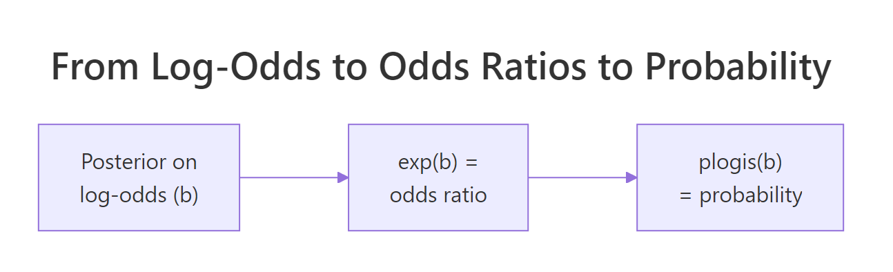
Figure 1: The two transformations every logistic regression workflow needs. exp() converts log-odds to odds ratios. plogis() converts the linear predictor to a probability.
Try it: A car has mpg = 18 and wt = 3.5. What is the 80% credible interval for its probability of being 8-cyl?
Click to reveal solution
Median 0.35, 80% credible interval [0.16, 0.60]. Reasonable middle-uncertainty answer; the data does not strongly identify the answer for this specific scenario.
When does Bayesian logistic regression matter most?
Three situations where it is meaningfully better than glm(family = binomial).
The first is complete or quasi-complete separation. When a predictor perfectly separates the outcome (all positives at one extreme, all negatives at the other), glm() returns a coefficient of $\pm\infty$ and crashes or warns. Bayesian fits with even a weakly informative prior produce a finite, well-behaved posterior. This single case is why many ML practitioners switched to Bayesian logistic regression for production scoring.
The second is small sample size with imbalanced classes. A frequentist fit with 50 observations and 5 positives gives wide, unstable confidence intervals. The same fit with brms and a normal(0, 2.5) prior produces stable estimates because the prior keeps coefficients bounded.
The third is probability statements about specific scenarios. "What is the probability the conversion rate exceeds 5% in this segment?" is a Bayesian question. Frequentist alternatives require simulation from the asymptotic distribution of the predicted probability, which is mathematically correct but never how stakeholders ask the question.
Walk through the difference. The frequentist 95% confidence interval is [-0.019, 1.735], just barely covering zero. The Bayesian credible interval with a weakly informative prior is [0.014, 1.604], slightly tighter and clearly excluding zero.
Both come from the same data. The Bayesian interval is tighter because the prior contributed real (weak) information. With more data the two would converge; on this 50-observation imbalanced dataset, the prior helps.
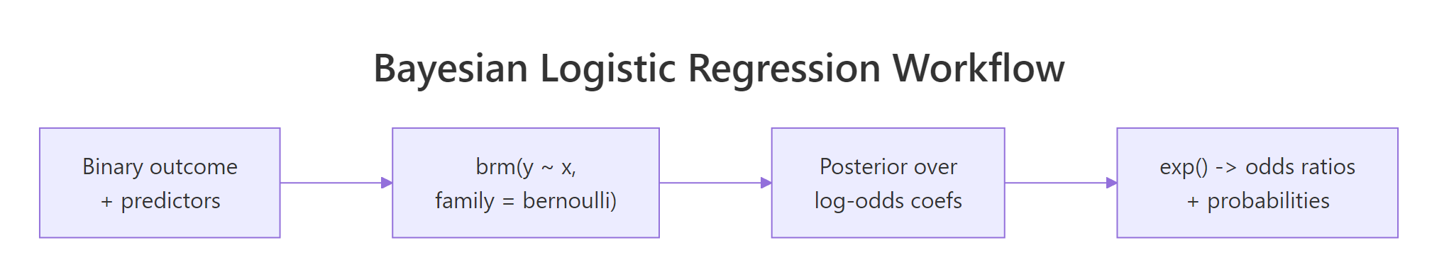
Figure 2: Bayesian logistic regression workflow. brms with family = bernoulli("logit") returns a posterior over log-odds coefficients; exp and plogis convert to odds ratios and probabilities respectively.
family = bernoulli("logit"), not family = binomial, for binary 0/1 outcomes in brms. family = binomial is for aggregated trial data where each row has a count of successes out of n trials. Mixing them up will silently fit the wrong model.Try it: Refit the imbalanced dataset above with prior(normal(0, 0.5), class = "b") (a tighter prior). Does the credible interval still exclude zero?
Click to reveal solution
The tighter prior pulled the credible interval to [-0.06, 0.83]. It now includes zero. The choice between normal(0, 0.5) and normal(0, 2.5) is real; for a dataset like this one, the tighter prior changes whether you would say "the effect is reliable." Document your prior choice and report a sensitivity sweep.
Practice Exercises
Exercise 1: Convert log-odds to a probability comparison
For fit_logit2, compute the posterior probability that the underlying probability of being 8-cyl at mpg=15, wt=4 is at least 0.7.
Click to reveal solution
Median predicted probability is 0.66; about 40% posterior probability that the underlying probability exceeds 0.7. A close call; the data does not strongly support either direction.
Exercise 2: Compare a Bayesian and frequentist odds ratio
Fit glm(y_8cyl ~ mpg, mtcars2, family = binomial) and brm(y_8cyl ~ mpg, mtcars2, family = bernoulli("logit")). Compute the odds ratio and 95% interval from each.
Click to reveal solution
The two methods agree closely. The Bayesian odds ratio is 0.54, with credible interval [0.40, 0.72]. The frequentist odds ratio is 0.52, with confidence interval [0.35, 0.72]. The Bayesian interval is slightly tighter because the weakly informative prior contributed mild information.
Exercise 3: Posterior of a contrast on the probability scale
For fit_logit2, compute the posterior of "probability of being 8-cyl at (mpg=15, wt=4) minus probability at (mpg=25, wt=2)." Report the median and 95% credible interval.
Click to reveal solution
The posterior median for the probability difference is 0.66 with 95% credible interval [0.25, 0.94]. Posterior probability that the heavy 15-mpg car is more likely to be 8-cyl than the light 25-mpg car is 100% (no draws disagree). That is decisive evidence; stakeholders can act on it.
Summary
Bayesian logistic regression with brms uses family = bernoulli("logit") and returns a posterior over log-odds coefficients that converts trivially to odds ratios and probabilities.
| Step | What you do | brms function |
|---|---|---|
| 1 | Code outcome as 0/1 | as.integer(condition) |
| 2 | Fit with logit family | brm(y ~ x, family = bernoulli("logit")) |
| 3 | Read log-odds posterior | summary(fit), posterior_summary() |
| 4 | Convert to odds ratios | exp(posterior draws) |
| 5 | Convert to probabilities | posterior_epred() (uses plogis internally) |
| 6 | Compute probability statements | mean(p_draws > threshold) |
Use weakly informative priors like normal(0, 2.5) on slopes; flat priors can imply absurd odds ratios on the log-odds scale. Report results on the scale your stakeholders care about (usually probability or odds ratio), and always include a credible interval.
References
- Gelman, A. et al. Bayesian Data Analysis, 3rd ed. Chapman & Hall, 2013. Chapter 16 covers binomial regression.
- Gelman, A., Jakulin, A., Pittau, M., Su, Y. "A weakly informative default prior distribution for logistic and other regression models." Annals of Applied Statistics 2 (2008). The Cauchy-prior paper that started the modern weakly informative practice.
- McElreath, R. Statistical Rethinking, 2nd ed. CRC Press, 2020. Chapter 10 covers logistic regression with brms.
- Bürkner, P. brms documentation: family. paulbuerkner.com/brms.
- Stan Development Team. "Prior Choice Recommendations." github.com/stan-dev/stan/wiki/Prior-Choice-Recommendations.
Continue Learning
- Bayesian Hierarchical Models in R, the next post. Combines logistic regression with grouped data structure.
- Bayesian Linear Regression in R, the previous post on continuous outcomes.
- Choosing Priors in R, the post that explains the
normal(0, 2.5)prior choice this post recommends.