Bayesian Statistics in R: Build Genuine Intuition Before Opening Stan or brms

By Selva Prabhakaran · Published May 9, 2026 · Last updated May 9, 2026

Bayesian statistics in R updates a prior belief about an unknown parameter with observed data, producing a posterior distribution you can plot, integrate, and reason about. Unlike frequentist methods that return a single point estimate plus a confidence interval whose interpretation trips up most students, the Bayesian workflow gives you the full probability curve over plausible parameter values, ready for decision-making.

How does Bayes' theorem turn data into a posterior?

Frequentist tools answer "what is the parameter?" with a point estimate and a confidence interval whose interpretation bends most readers' minds. Bayesian inference flips the question. You start with a prior belief about the parameter, observe data, and end with a posterior distribution: a probability curve over every plausible value. This section shows that update happen in a single line of base R using the Beta-Binomial pair, the simplest example of an analytic posterior.

The math behind every Bayesian update is one line:

$$ p(\theta \mid \text{data}) \;\propto\; p(\text{data} \mid \theta) \cdot p(\theta) $$

Where: $p(\theta)$ is the prior, $p(\text{data} \mid \theta)$ is the likelihood, and $p(\theta \mid \text{data})$ is the posterior. The proportional sign hides a normalizing constant that does not affect the shape of the curve.

Suppose you flip a possibly-biased coin 100 times and see 65 heads. You want to estimate the unknown success probability theta. A Beta(2, 2) prior is mildly skeptical of extreme values, gently centered at 0.5. The posterior comes out in closed form because the Beta family is conjugate to the Binomial likelihood, meaning the posterior stays in the Beta family.

RBeta-Binomial posterior from 100 flips

n <- 100 # total flips k <- 65 # heads observed alpha_prior <- 2 # prior shape parameters beta_prior <- 2 # ... encoding "fair-ish, but uncertain" alpha_post <- alpha_prior + k # closed-form posterior shape beta_post <- beta_prior + n - k # ... thanks to Beta-Binomial conjugacy post_mean <- alpha_post / (alpha_post + beta_post) cri <- qbeta(c(0.025, 0.975), alpha_post, beta_post) post_mean #> [1] 0.6442308 cri #> [1] 0.5497073 0.7321076

The posterior is Beta(67, 37). Its mean of 0.644 sits between the prior mean of 0.5 and the data proportion of 0.65, gently pulled toward 0.5 by the prior's weight. The 95% credible interval [0.55, 0.73] is the range that contains 95% of the posterior probability mass. That is the interpretation people incorrectly give a frequentist confidence interval.

The Bayesian update workflow

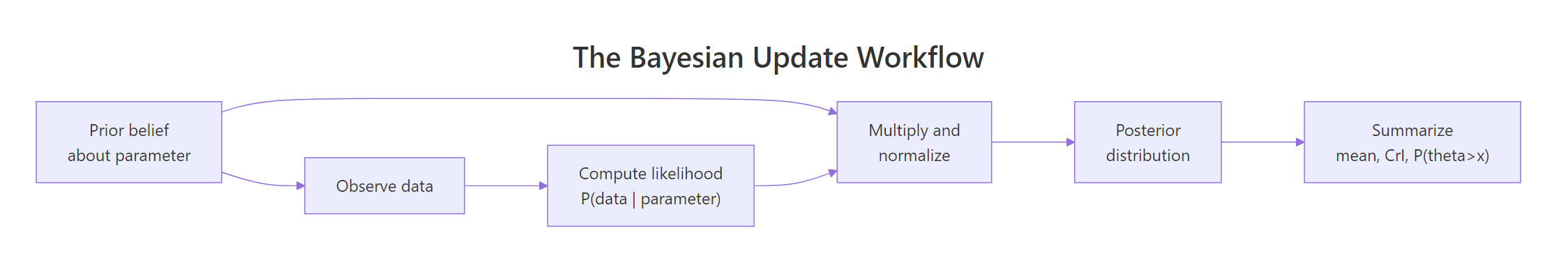
Figure 1: The Bayesian update workflow. Prior plus data give a posterior, which you then summarize.

Key Insight

The posterior is the prior reweighted by the likelihood. No exotic computation, just multiplication and renormalization. The Beta-Binomial pair gives you the answer in closed form because the Beta family is conjugate to the Binomial, meaning the posterior stays in the Beta family.

Try it: Repeat the calculation with a much tighter prior, Beta(20, 20). What does the posterior mean become and why?

RYour turn: tighten the prior

ex_alpha <- 20 # try a tight prior ex_beta <- 20 # compute the posterior shape parameters and posterior mean here # ex_alpha_post <- ? # ex_beta_post <- ? # ex_post_mean <- ? #> Expected: posterior mean closer to 0.5 than 0.65

Click to reveal solution

RTighter prior solution

ex_alpha_post <- ex_alpha + k ex_beta_post <- ex_beta + n - k ex_post_mean <- ex_alpha_post / (ex_alpha_post + ex_beta_post) ex_post_mean #> [1] 0.6071429

A Beta(20, 20) prior is equivalent to having seen 38 prior flips with 19 heads. Adding the new 100 flips gives a posterior that is pulled noticeably back toward 0.5. A stronger prior carries more weight against the same data, that is the lesson here.

What does a prior actually encode?

A prior is just a probability distribution over the parameter. Anything you can put on a curve, you can use as a prior. The Beta family is convenient for proportions because it lives on [0, 1] and supports two intuitive shape parameters that act like pseudo-counts of prior successes and failures. Three Beta priors illustrate the spectrum from ignorance to strong belief.

RThree priors plotted on one panel

theta_grid <- seq(0, 1, length.out = 200) plot(theta_grid, dbeta(theta_grid, 1, 1), type = "l", lwd = 2, ylim = c(0, 6), xlab = expression(theta), ylab = "density", main = "Three priors over a proportion") lines(theta_grid, dbeta(theta_grid, 20, 20), lwd = 2, col = "steelblue") lines(theta_grid, dbeta(theta_grid, 2, 5), lwd = 2, col = "tomato") legend("topright", lwd = 2, col = c("black", "steelblue", "tomato"), legend = c("Beta(1,1) uniform", "Beta(20,20) tight at 0.5", "Beta(2,5) skewed low"))

Beta(1, 1) is flat: every value of theta is equally plausible before seeing data. Beta(20, 20) is tight around 0.5: a strong belief that the coin is fair. Beta(2, 5) is skewed low: a belief that small values of theta are more likely. Each shape encodes a different domain assumption, and each will pull the posterior in a different direction.

You often have a substantive belief such as "I think theta is between 0.4 and 0.6 with about 90% probability." That language has a direct Beta translation. Search for shape parameters whose 5th and 95th percentiles match the beliefs. A symmetric, moderately tight Beta(45, 45) lands close.

RQuantile-based prior elicitation

qbeta(c(0.05, 0.95), 45, 45) #> [1] 0.4133497 0.5866503

A Beta(45, 45) prior places 90% of its mass between 0.41 and 0.59, a near-perfect match for the stated belief. If you wanted a less tight prior, lower both shape parameters; for a more confident prior, raise them. This is how to translate qualitative belief into a quantitative prior without throwing darts.

Tip

Pick a prior whose shape matches your prior belief, document the choice, and plan to report sensitivity. Beta(2, 2) is mildly skeptical of extreme values; Beta(1, 1) is informationless; Beta(50, 50) is hard to budge. Match the prior to the belief, then check how much the answer changes if you nudge the prior.

Try it: Encode the belief "I think theta is around 0.7 with mild uncertainty" as Beta shape parameters. A good answer keeps most mass in the [0.6, 0.8] range.

RYour turn: encode a belief at 0.7

ex_alpha2 <- 0 # replace ex_beta2 <- 0 # replace # Verify with: qbeta(c(0.05, 0.95), ex_alpha2, ex_beta2) #> Expected: 90% interval roughly [0.6, 0.8]

Click to reveal solution

RBelief-at-0.7 solution

ex_alpha2 <- 35 ex_beta2 <- 15 qbeta(c(0.05, 0.95), ex_alpha2, ex_beta2) #> [1] 0.5901019 0.8003617

Beta(35, 15) has mean 35/50 = 0.7 with 90% of its mass between 0.59 and 0.80. The ratio alpha/(alpha+beta) controls the center; the sum alpha+beta controls how tight the curve is. Combine those two levers to encode any belief on [0,1].

How do prior and likelihood combine into a posterior?

The likelihood is a function of the parameter, given fixed data. It is not itself a probability distribution over theta, just a curve showing which theta values are most consistent with what you saw. Multiply the likelihood curve by the prior curve, normalize so the area is 1, and you have the posterior. Plotting all three on the same axes makes the arithmetic visual.

RPrior, likelihood, posterior on one panel

likelihood_vals <- dbinom(k, size = n, prob = theta_grid) par(mfrow = c(1, 3), mar = c(4, 4, 3, 1)) plot(theta_grid, dbeta(theta_grid, alpha_prior, beta_prior), type = "l", lwd = 2, main = "Prior Beta(2, 2)", xlab = expression(theta), ylab = "density") plot(theta_grid, likelihood_vals, type = "l", lwd = 2, col = "tomato", main = "Likelihood Binomial(n=100, k=65)", xlab = expression(theta), ylab = "L(theta)") plot(theta_grid, dbeta(theta_grid, alpha_post, beta_post), type = "l", lwd = 2, col = "steelblue", main = "Posterior Beta(67, 37)", xlab = expression(theta), ylab = "density") par(mfrow = c(1, 1))

The likelihood peaks at the maximum likelihood estimate, exactly k/n = 0.65. The prior peaks at 0.5. The posterior peaks slightly below 0.65, pulled toward the prior in proportion to the prior's tightness. With a weak prior and large n, the posterior almost coincides with the likelihood.

Beta-Binomial conjugate update

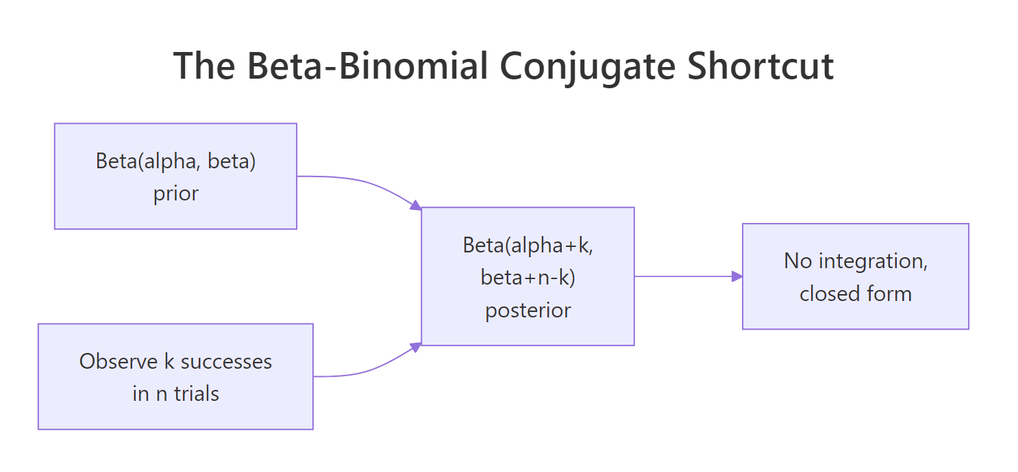
Figure 2: Beta-Binomial conjugate. Closed-form posterior parameters absorb counts of observed successes and failures.

Key Insight

The posterior always lies between the prior and the likelihood, weighted by their relative confidence. A flat prior gives you back the likelihood. A point-mass prior ignores the data entirely. Real priors live in between, and the data nudges the answer accordingly.

Try it: Suppose you observed 20 heads in 100 flips instead of 65. Recompute the posterior parameters and the posterior mean.

RYour turn: shift the data

ex_k_new <- 20 # compute new alpha_post, beta_post, and posterior mean #> Expected: posterior mean near 0.21

Click to reveal solution

RShifted-data solution

ex_alpha_post_new <- alpha_prior + ex_k_new ex_beta_post_new <- beta_prior + n - ex_k_new ex_alpha_post_new / (ex_alpha_post_new + ex_beta_post_new) #> [1] 0.2115385

The posterior peaks near 0.21, just above the data proportion 0.20, slightly pulled toward 0.5 by the prior. The shape and the location of the curve both follow the data, while the prior modulates the pull.

How does the posterior shift as more data arrives?

A common worry about Bayesian methods is "what if I pick the wrong prior?" The honest answer: with enough data, the prior gets washed out. Likelihood scales with n, prior does not, so the posterior shifts toward the data as n grows. Showing this with a deliberately bad prior makes the point concrete.

RPosterior with n = 10, 100, 1000 against a wrong prior

true_theta <- 0.7 # the truth we are trying to recover sims <- list( small = list(n = 10, k = round(0.7 * 10)), # 7 / 10 medium = list(n = 100, k = round(0.7 * 100)), # 70 / 100 large = list(n = 1000, k = round(0.7 * 1000)) # 700/ 1000 ) wrong_alpha <- 80 # a stubborn prior centered at 0.8 ... wrong_beta <- 20 # ... that disagrees with the truth plot(theta_grid, dbeta(theta_grid, wrong_alpha, wrong_beta), type = "l", lwd = 2, ylim = c(0, 30), xlab = expression(theta), ylab = "density", main = "Posterior shifts toward the truth as n grows") abline(v = true_theta, lty = 2) cols <- c("tomato", "orange", "steelblue") for (i in seq_along(sims)) { s <- sims[[i]] lines(theta_grid, dbeta(theta_grid, wrong_alpha + s$k, wrong_beta + s$n - s$k), lwd = 2, col = cols[i]) } legend("topleft", lwd = 2, col = c("black", cols), legend = c("Wrong prior Beta(80,20)", "n=10", "n=100", "n=1000"))

The prior peaks at 0.8 and refuses to budge much for n=10. By n=100 the posterior straddles 0.75. By n=1000 it has converged tightly around the true 0.7. The posterior peak migrates from prior toward truth as the data accumulates.

A subtler property of Bayes' theorem is that updates are order-independent. If you observe one batch, then another, then update sequentially, the result is mathematically identical to combining everything and updating once. The check below verifies that.

RSequential vs one-shot update

batch1 <- list(n = 50, k = 35) batch2 <- list(n = 50, k = 40) # Sequential: update after each batch seq_first <- c(alpha = 1 + batch1$k, beta = 1 + batch1$n - batch1$k) # Beta(36, 16) seq_second <- c(alpha = seq_first["alpha"] + batch2$k, beta = seq_first["beta"] + batch2$n - batch2$k) # Beta(76, 26) # One-shot: combine batches and update once seq_combined <- c(alpha = 1 + batch1$k + batch2$k, beta = 1 + batch1$n + batch2$n - batch1$k - batch2$k) seq_second #> alpha.alpha beta.beta #> 76 26 seq_combined #> alpha beta #> 76 26

Both paths land on Beta(76, 26). Sequential and one-shot updates are mathematically identical, which is why Bayesian methods fit naturally to streaming data: every new observation just nudges the existing posterior into a new posterior of the same family.

Note

Bayes' theorem is order-independent and incremental. Observe one row at a time, ten at a time, or a million at a time, the math gives the same answer. That makes Bayesian updates the natural model for online learning and experimental design.

Try it: Start from a uniform Beta(1, 1) prior, observe n = 1000 with k = 700 (true theta = 0.7). Where does the posterior peak, and how tight is the 95% credible interval?

RYour turn: uniform prior + n = 1000

ex_alpha_unif <- 0 # replace ex_beta_unif <- 0 # replace # ex_alpha_unif / (ex_alpha_unif + ex_beta_unif) # qbeta(c(0.025, 0.975), ex_alpha_unif, ex_beta_unif) #> Expected: posterior tightly peaked near 0.7

Click to reveal solution

RUniform prior + n = 1000 solution

ex_alpha_unif <- 1 + 700 ex_beta_unif <- 1 + 1000 - 700 ex_alpha_unif / (ex_alpha_unif + ex_beta_unif) #> [1] 0.6993014 qbeta(c(0.025, 0.975), ex_alpha_unif, ex_beta_unif) #> [1] 0.6705486 0.7269683

A uniform prior plus 1000 observations gives a posterior whose mean is essentially the data proportion, with a 95% credible interval roughly +/- 0.03 around the truth. With this much data, the choice of weak prior barely matters.

How do we summarize a posterior in R?

A posterior is a curve, not a number. To report or act on it you reduce it to a few summaries: a central estimate, an interval that captures most of the mass, and the probability of any event of interest. R provides every Beta family helper you need: dbeta, pbeta, qbeta, rbeta.

RMean, mode, credible interval, P(theta > 0.5)

post_mean #> [1] 0.6442308 post_mode <- (alpha_post - 1) / (alpha_post + beta_post - 2) # valid for alpha,beta > 1 post_mode #> [1] 0.6470588 cri #> [1] 0.5497073 0.7321076 p_gt_half <- 1 - pbeta(0.5, alpha_post, beta_post) p_gt_half #> [1] 0.9979088 p_hat <- k / n freq_ci <- p_hat + c(-1, 1) * qnorm(0.975) * sqrt(p_hat * (1 - p_hat) / n) freq_ci #> [1] 0.5565097 0.7434903

The 95% credible interval [0.55, 0.73] is similar in width to the frequentist Wald CI [0.56, 0.74], but the interpretation differs sharply. The Bayesian statement is "given my prior and the data, there is a 95% probability that theta is in this interval." The frequentist statement is the multi-step contortion most students stumble over. The posterior probability of 0.998 that theta exceeds 0.5 is the kind of statement decision-makers can act on directly.

Note

The credible interval has the interpretation people want from a confidence interval. That alone is worth the price of admission to Bayesian thinking. A posterior probability of 0.998 that theta exceeds 0.5 is far more communicable than "p < 0.001."

Try it: What is the posterior probability that theta > 0.6?

RYour turn: P(theta > 0.6)

# use 1 - pbeta() with alpha_post and beta_post # ex_p <- ? #> Expected: a value between 0.7 and 0.9

Click to reveal solution

RTail-probability solution

ex_p <- 1 - pbeta(0.6, alpha_post, beta_post) ex_p #> [1] 0.8164234

There is roughly an 82% posterior probability that theta exceeds 0.6 given this prior and these data. Combined with the credible interval, you can quote any tail probability the stakeholder cares about.

What if my prior matters? How do I check sensitivity?

The honest answer to "what if my prior is wrong?" is to try several reasonable priors and see whether the conclusion changes. If three plausible priors give similar posteriors, you have a robust answer. If they give materially different posteriors, that is itself a finding to report alongside the analysis. The check is cheap with conjugate priors.

RPrior sensitivity comparison

priors <- list( skeptical = c(alpha = 2, beta = 5), # leans toward small theta uniform = c(alpha = 1, beta = 1), # informationless optimistic = c(alpha = 8, beta = 2) # leans toward large theta ) posterior_summary <- t(sapply(priors, function(p) { ap <- p["alpha"] + k bp <- p["beta"] + n - k c(post_mean = ap / (ap + bp), cri_low = qbeta(0.025, ap, bp), cri_high = qbeta(0.975, ap, bp), p_above_half = 1 - pbeta(0.5, ap, bp)) })) round(posterior_summary, 3) #> post_mean.alpha cri_low cri_high p_above_half #> skeptical 0.626 0.530 0.717 0.992 #> uniform 0.647 0.553 0.736 0.998 #> optimistic 0.664 0.572 0.751 0.999

All three priors produce posterior means within 0.04 of each other and 95% credible intervals that overlap heavily. The posterior probability that theta > 0.5 ranges from 0.992 to 0.999, well above any reasonable decision threshold. The conclusion that theta likely exceeds 0.5 is robust to a reasonable change of prior. That is exactly what you want to be able to report.

When to reach for MCMC

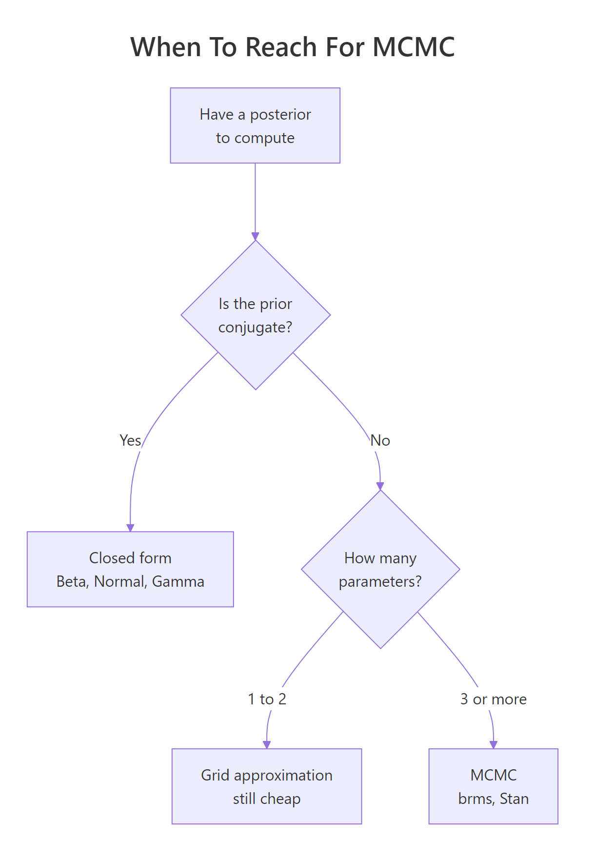
Figure 3: When to reach for MCMC. The decision tree from conjugate to grid to sampling.

Tip

Prior sensitivity reporting is the credibility currency of Bayesian analysis. Always show the answer under your stated prior plus a couple of reasonable alternatives. If the conclusions agree directionally, you have a robust result. If they disagree, that is the finding.

Try it: With a smaller dataset (n = 20, k = 15), check sensitivity under three prior strengths: Beta(2, 2), Beta(50, 50), Beta(200, 200). How much do posterior means differ?

RYour turn: vary prior strength

ex_n2 <- 20 ex_k2 <- 15 ex_strengths <- list(weak = c(2, 2), medium = c(50, 50), strong = c(200, 200)) # compute posterior mean under each prior #> Expected: weak posterior near 0.75, strong posterior near 0.55

Click to reveal solution

RVary prior strength solution

sapply(ex_strengths, function(p) { ap <- p[1] + ex_k2 bp <- p[2] + ex_n2 - ex_k2 ap / (ap + bp) }) #> weak medium strong #> 0.7083333 0.6500000 0.5568182

With only 20 observations, the prior carries real weight. The weak Beta(2, 2) prior lets the data dominate (posterior mean 0.71 against data 0.75). The strong Beta(200, 200) prior pulls hard toward 0.5 (posterior mean 0.56). With small samples, prior choice is consequential and you must report sensitivity.

When do we need MCMC instead of analytic posteriors?

The Beta-Binomial pair is conjugate, meaning the posterior stays in the same Beta family as the prior. Conjugate priors exist for several common likelihoods (Normal-Normal, Gamma-Poisson) and they all give closed-form posteriors. Once you leave that small family, or once you have more than a couple of unknown parameters, the integral that normalizes the posterior becomes intractable. Grid approximation on a 2-parameter Normal model shows the limit of brute force.

RGrid approximation for Normal mean and standard deviation

set.seed(42) y_obs <- rnorm(20, mean = 5, sd = 1.5) # 20 observations from a Normal mu_grid <- seq(3, 7, length.out = 80) # 80 candidate means sigma_grid <- seq(0.5, 3, length.out = 80) # 80 candidate sds post_grid <- outer(mu_grid, sigma_grid, function(m, s) { loglik <- sapply(seq_along(m), function(i) sum(dnorm(y_obs, mean = m[i], sd = s[i], log = TRUE))) exp(loglik - max(loglik)) # rescale for numerical safety }) post_grid <- post_grid / sum(post_grid) # normalize # posterior mean for mu, marginalizing over sigma mu_post_mean <- sum(mu_grid * rowSums(post_grid)) mu_post_mean #> [1] 5.124375

For two unknowns we computed 80 x 80 = 6,400 posterior values, which fits in memory. Add a third parameter and you need 80^3 = 512,000 cells. Add a fourth and you are in the millions. This combinatorial blow-up is why MCMC exists: it samples from the posterior without ever computing it on a grid.

Tip

brms and Stan are MCMC engines under the hood, plus convenient model syntax. The intuition you built here, prior plus likelihood gives posterior, transfers directly. MCMC just produces samples instead of a closed form, and the same summaries (mean, credible interval, tail probability) work on samples.

Try it: Roughly how many cells does grid approximation need for 5 parameters at 50 points each?

RYour turn: cost of 5 parameters

ex_d <- 5 # number of parameters # total cells needed at 50 points each #> Expected: a number above 300 million

Click to reveal solution

R5-parameter grid cost

50 ^ ex_d #> [1] 312500000

Over 312 million cells. The cost grows exponentially in the dimension. By six or seven parameters even cluster-scale grids are infeasible, and that is exactly the wall MCMC was invented to scale past.

Practice Exercises

Exercise 1: Twitter survey

A Twitter survey asks 50 users whether they like a new feature; 32 say yes. Use a Beta(2, 2) prior to compute the posterior, the posterior mean, and a 95% credible interval over the true approval rate.

RExercise 1 starter

tw_n <- 50 tw_k <- 32 # compute tw_post_alpha, tw_post_beta, tw_mean, and a 95% CrI

Click to reveal solution

RExercise 1 solution

tw_post_alpha <- 2 + tw_k tw_post_beta <- 2 + tw_n - tw_k tw_mean <- tw_post_alpha / (tw_post_alpha + tw_post_beta) tw_cri <- qbeta(c(0.025, 0.975), tw_post_alpha, tw_post_beta) tw_mean #> [1] 0.6296296 tw_cri #> [1] 0.4928577 0.7536919

Posterior is Beta(34, 20), mean 0.63, 95% CrI [0.49, 0.75]. The credible interval includes 0.5, so you cannot yet rule out the possibility that the feature is no better than a coin flip.

Exercise 2: Sequential update equals one-shot update

Observe two batches of 50 flips: 35 heads in the first, 40 heads in the second. Show that updating once after each batch gives the same posterior as combining everything and updating once with n = 100, k = 75. Use a Beta(1, 1) prior.

RExercise 2 starter

# Stage 1: prior Beta(1,1), data k=35 in n=50 -> posterior_1 # Stage 2: prior posterior_1, data k=40 in n=50 -> posterior_2 # One-shot: prior Beta(1,1), data k=75 in n=100 -> posterior_oneshot

Click to reveal solution

RExercise 2 solution

seq2_first <- c(alpha = 1 + 35, beta = 1 + 50 - 35) # Beta(36, 16) seq2_second <- c(alpha = seq2_first["alpha"] + 40, beta = seq2_first["beta"] + 50 - 40) # Beta(76, 26) seq2_combined <- c(alpha = 1 + 75, beta = 1 + 100 - 75) # Beta(76, 26) seq2_second #> alpha.alpha beta.beta #> 76 26 seq2_combined #> alpha beta #> 76 26

Both paths land on Beta(76, 26). Bayes' theorem is order-independent and incremental.

Exercise 3: Three-prior sensitivity

You observe 20 successes in 30 trials. Compute posteriors and posterior P(theta > 0.5) under three priors: Beta(1, 1), Beta(2, 5), Beta(8, 2). Report all three posterior means and tail probabilities. Are the conclusions robust?

RExercise 3 starter

n_e <- 30 k_e <- 20 ex3_priors <- list(uniform = c(1, 1), skeptical = c(2, 5), optimistic = c(8, 2)) # compute posterior mean and P(theta > 0.5) under each prior

Click to reveal solution

RExercise 3 solution

ex3_summary <- t(sapply(ex3_priors, function(p) { ap <- p[1] + k_e bp <- p[2] + n_e - k_e c(post_mean = ap / (ap + bp), p_gt_half = 1 - pbeta(0.5, ap, bp)) })) round(ex3_summary, 3) #> post_mean p_gt_half #> uniform 0.656 0.953 #> skeptical 0.595 0.846 #> optimistic 0.700 0.987

All three priors agree directionally that theta probably exceeds 0.5 (tail probability between 0.85 and 0.99). The skeptical prior cools the conclusion by about 0.1, the optimistic prior warms it. With only 30 observations the prior matters, but the directional conclusion survives all three reasonable priors.

Complete Example: Customer Satisfaction Survey

A SaaS company surveys 200 customers and finds 132 say they would recommend the product. Marketing wants to claim the recommendation rate is "above 60%." Quantify that claim under three priors: a skeptical Beta(2, 5), an uninformative Beta(1, 1), and an optimistic Beta(8, 2). Report posterior summaries and the posterior probability that theta > 0.6 under each.

RCustomer satisfaction with three priors

cs_n <- 200 cs_k <- 132 cs_priors <- list( skeptical = c(alpha = 2, beta = 5), uniform = c(alpha = 1, beta = 1), optimistic = c(alpha = 8, beta = 2) ) cs_summary <- t(sapply(cs_priors, function(p) { ap <- p["alpha"] + cs_k bp <- p["beta"] + cs_n - cs_k c(post_mean = ap / (ap + bp), cri_low = qbeta(0.025, ap, bp), cri_high = qbeta(0.975, ap, bp), p_above_0.6 = 1 - pbeta(0.6, ap, bp)) })) round(cs_summary, 3) #> post_mean.alpha cri_low.alpha cri_high.alpha p_above_0.6.alpha #> skeptical 0.646 0.578 0.710 0.909 #> uniform 0.658 0.591 0.723 0.950 #> optimistic 0.667 0.601 0.730 0.975

All three priors give posterior probability above 90% that the true recommendation rate exceeds 60%. The skeptical prior is the most conservative (90.9%), and even it strongly supports marketing's claim. The conclusion is robust to a reasonable change of prior, which is exactly the kind of report a careful Bayesian analyst delivers: a primary estimate plus an explicit sensitivity check.

Summary

Question	Frequentist answer	Bayesian answer
Best estimate of theta	k/n point estimate	Posterior mean (Beta(alpha+k, beta+n-k) for proportions)
Uncertainty	95% confidence interval	95% credible interval
Interpretation of interval	"If we repeated the experiment, 95% of such intervals would cover theta."	"Given prior and data, there is a 95% probability that theta is in this interval."
Probability of an event	Not well-defined (theta is fixed, not random)	Computed by integrating the posterior
What you input	Data only	Prior plus data
What you output	Single number plus CI	Full probability distribution
Robustness check	Power, replication	Prior sensitivity analysis

References

McElreath, R. Statistical Rethinking, 2nd ed. Chapman & Hall, 2020. Chapters 1-2 build the prior-likelihood-posterior intuition with worked simulations.
Gelman, A., Carlin, J. B., Stern, H. S. et al. Bayesian Data Analysis, 3rd ed. Chapman & Hall, 2013. Chapters 1-2 cover the foundations.
Johnson, A. A., Ott, M. Q., Dogucu, M. Bayes Rules! An Introduction to Applied Bayesian Modeling. Chapman & Hall, 2022. Open access at bayesrulesbook.com. Chapter 3 is the canonical Beta-Binomial reference.
CRAN Task View: Bayesian Inference. cran.r-project.org/web/views/Bayesian.html. Curated list of R packages for Bayesian analysis.
Coghlan, A. A Little Book of R for Bayesian Statistics. a-little-book-of-r-for-bayesian-statistics.readthedocs.io. Practical proportion-estimation worked examples.
Gelman, A. and the Stan team. "Prior choice recommendations." github.com/stan-dev/stan/wiki/Prior-Choice-Recommendations. The community standard for principled prior choice.
R-bloggers. "An Intuitive Look at Binomial Probability in a Bayesian Context." r-bloggers.com, 2020. Gold-merchant analogy and grid approximation animation.

Continue Learning

Bayes' Theorem in R, the discrete foundation, worked through medical-test reasoning.
Gamma & Beta Distributions in R, full mechanics of the Beta family used as priors here.
Maximum Likelihood Estimation in R, the frequentist counterpart to compare against the Bayesian workflow.

Bayesian Statistics in R: Build Genuine Intuition Before Opening Stan or brms

How does Bayes' theorem turn data into a posterior?

What does a prior actually encode?

How do prior and likelihood combine into a posterior?

How does the posterior shift as more data arrives?

How do we summarize a posterior in R?

What if my prior matters? How do I check sensitivity?

When do we need MCMC instead of analytic posteriors?

Practice Exercises

Exercise 1: Twitter survey

Exercise 2: Sequential update equals one-shot update

Exercise 3: Three-prior sensitivity

Complete Example: Customer Satisfaction Survey

Summary

References

Continue Learning

Related Tutorials