Bootstrap in R: boot Package, CI & Hypothesis Tests Without Assumptions

The bootstrap resamples your data with replacement to estimate confidence intervals and run hypothesis tests without assuming a normal distribution. The boot package in R turns the workflow into two calls: boot() to generate replicates and boot.ci() to extract BCa, percentile, basic, or normal intervals.

How do you bootstrap in R with the boot package?

The fastest way to see the bootstrap in action is to compute a 95% CI for a statistic that has no clean textbook formula. The median of a small sample fits: there is no closed-form CI, and its sampling distribution is rarely normal. Here is the entire bootstrap pipeline for the median MPG in mtcars.

The pattern is always the same: define a statistic function that takes data and an index vector, hand it to boot(), then pass the result to boot.ci().

Two thousand resamples produced two 95% intervals for the median. The percentile CI runs from 16.4 to 21.4 MPG. The BCa CI runs slightly wider on the upper end (22.05) because BCa adjusts for skewness in the bootstrap distribution. Both agree the true population median plausibly sits in this range, and you got there without a single distributional assumption.

The statistic function has a strict signature: first argument is the data, second is an integer index vector. Inside the function, d[i] (for vectors) or d[i, ] (for data frames) builds the bootstrap sample. boot() calls your function R times with random indices and stores every replicate in boot_out$t.

Why does bootstrap work without distributional assumptions?

Classical confidence intervals lean on a formula like $\bar{x} \pm 1.96 \cdot s/\sqrt{n}$. That formula is correct only if the sampling distribution of the mean is approximately normal, which itself requires assumptions about the population or a sufficiently large sample. The bootstrap sidesteps that machinery by replacing "what would the population look like?" with "the sample is the best guess we have for the population."

Mathematically, the bootstrap uses the empirical distribution function, the discrete distribution that puts probability $1/n$ on each observed data point. Sampling with replacement from your data is sampling from that empirical distribution. As $n$ grows, it converges to the true population, so resampled statistics converge to true sampling statistics.

$$\hat{F}_n(x) = \frac{1}{n} \sum_{i=1}^{n} \mathbb{1}\{x_i \leq x\}$$

Where:

• $\hat{F}_n(x)$ = the empirical distribution function evaluated at $x$
• $n$ = sample size
• $\mathbb{1}\{x_i \leq x\}$ = an indicator that is 1 if $x_i \leq x$, else 0

If you are not interested in the math, skip to the next paragraph. The practical takeaway is unchanged: every replicate is a "what could my sample have looked like?" scenario, and the spread of replicates is the spread of the statistic.

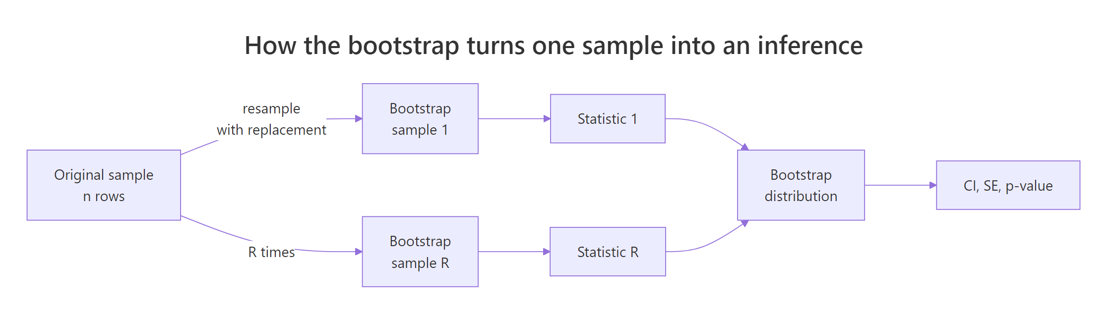
Figure 1: The bootstrap resamples one observed sample many times to build a distribution of any statistic.

The bootstrap distribution is just the histogram of boot_out$t. Plotting it tells you the shape of the sampling distribution, the centre (your point estimate), and the spread (the standard error).

The peak of the histogram lines up with the observed median (red line), confirming the bootstrap is unbiased on average. The width of the histogram is the bootstrap standard error: roughly the standard deviation of the replicates. If you saw a wildly skewed shape or two distinct modes, you would know that a normal-based CI would be wrong here, even before computing the interval.

Which bootstrap confidence interval should you use?

The boot package offers five interval types: percentile, basic, normal, BCa, and studentized. The first four are one-line calls; studentized needs an extra variance estimate per replicate. For most applied work, the choice narrows to BCa or percentile.

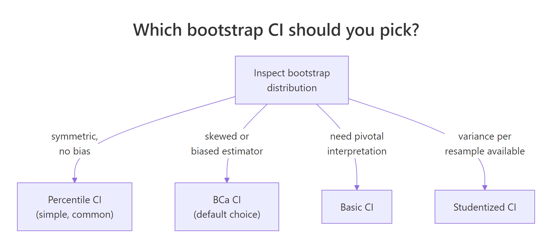
Figure 2: A quick decision rule for picking the right boot.ci() type.

Asking for all four at once is a quick way to compare them on the same data. A large gap between them is a warning that one or more is misbehaving.

Three of the four CIs share their lower bound (16.4) because the bootstrap distribution of the median has a hard floor near that value. Their upper bounds differ: BCa stretches to 22.05 while percentile and basic stop at 21.40. BCa is doing what it was designed for, correcting for the asymmetric tail of the distribution. The Normal CI extends below 16.40, which is impossible since the percentile bound is 16.40, signalling that a Gaussian approximation does not fit this distribution.

You can also pull out just the BCa interval as a numeric vector. The bca element holds the level, the bootstrap quantile indices, and the lower and upper bounds in its last two columns.

How do you run a bootstrap hypothesis test in R?

There are two common routes. The CI route is the simplest: bootstrap a CI for the test statistic and reject the null at level $\alpha$ if the null value falls outside the $1-\alpha$ CI. The shift route is more direct: simulate replicates that satisfy the null, then count how often they are at least as extreme as the observed statistic.

The CI route shines for "is the mean of group A different from group B?" questions. Bootstrap a CI for the difference in means; if zero is outside the CI, reject the null of equal means.

The 95% BCa CI for the difference in mean MPG (4-cyl minus 6-cyl) runs from 4.74 to 9.83. Zero is far outside. We reject the null that the two cylinder groups have the same mean MPG, with the same conclusion you would get from a t-test, but without the equal-variance or normality assumption.

The shift route gives you a proper bootstrap p-value. Centre the replicates so their mean is zero (the null), then count how many of them are at least as far from zero as the observed difference.

The two-sided p-value is effectively zero, again rejecting the null. This is the same logic as a permutation test: build a distribution under H0 and ask how surprising the data are. The CI route asks the dual question, "is the null inside the plausible range?", and gives the same answer when the test is well-defined.

When does bootstrap fail and how do you spot it?

The bootstrap is not magic. Three failure modes show up often enough that you should know what they look like.

The first is tiny samples. With $n < 10$, there are very few distinct resamples and the bootstrap distribution becomes blocky and unreliable. The CI you get back is overconfident.

The second is boundary statistics. The maximum, minimum, and other extremes have a sampling distribution that piles up against the observed value. Bootstrap mimics this pile-up and underestimates the true uncertainty.

The histogram is a single spike at the observed maximum with a sparse tail to its left. The bootstrap can never produce a value larger than the observed maximum, because the maximum of a resample with replacement cannot exceed the original maximum. So the upper tail is zero by construction, and any CI would be misleading. For boundary statistics, look at parametric methods or order-statistic theory instead.

The third is dependent data. If your observations are a time series, ordinary bootstrap destroys the autocorrelation. Use tsboot() from the same package with the block bootstrap (sim = "fixed" or "geom") to preserve local dependence.

How do you run a stratified bootstrap?

When the data has groups and you want each replicate to preserve group sizes, pass a strata vector to boot(). This is essential when groups have very different sizes or behaviours and you do not want bootstrap replicates that accidentally drop one group.

The example below estimates the ratio of mean MPG between automatic (am = 1) and manual (am = 0) cars in mtcars, with strata = mtcars$am so each replicate keeps the original 13 automatic and 19 manual cars.

The 95% BCa CI for the ratio runs from 1.13 to 1.62. Because the entire CI is above 1, automatic-transmission cars get more MPG on average than manual-transmission ones in this dataset, by a factor of 13% to 62%. Without strata, some replicates would have very few automatic cars, inflating the variance and the CI width.

Practice Exercises

Exercise 1: Bootstrap a regression slope

Bootstrap a 95% BCa CI for the slope of lm(mpg ~ wt, data = mtcars). Save the boot result to my_boot_slope and print the BCa interval.

Exercise 2: Bootstrap p-value for "median equals 20"

Compute a two-sided bootstrap p-value for the null that the median of mtcars$mpg equals 20. Centre the replicates around 20 and count how often the centred replicates are at least as far from 20 as the observed median is.

Complete Example

A common applied use case is reporting a 95% CI for a regression coefficient when you do not trust the residual normality. Here is the full pipeline applied to the slope of mpg ~ wt. The code is one block: define statistic, run boot(), extract BCa CI, and visualise.

The 95% BCa CI for the slope is $(-7.42, -3.81)$. In plain English, every extra 1000 lbs of car weight is associated with a drop of between 3.81 and 7.42 MPG, with 95% confidence. Because the entire interval is below zero, the relationship is unambiguous and the conclusion does not depend on Gaussian residual assumptions.

Summary

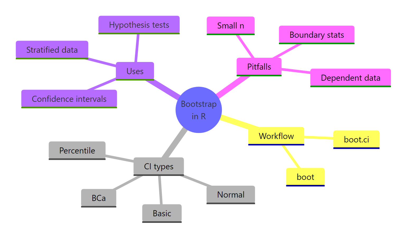
Figure 3: Bootstrap in R at a glance: workflow, CI types, uses, and pitfalls.

Three rules of thumb to remember:

1. Default to BCa intervals when in doubt; they correct for bias and skew.
2. Always set a seed and use R >= 1000 for stable CIs (R >= 5000 for p-values).
3. Skip the bootstrap for boundary statistics (max, min) and dependent data without blocks.

References

1. Efron, B. (1979). Bootstrap Methods: Another Look at the Jackknife. Annals of Statistics, 7(1). Link
2. Davison, A. C. & Hinkley, D. V. (1997). Bootstrap Methods and Their Application. Cambridge University Press. Link
3. Canty, A. & Ripley, B. boot: Bootstrap Functions (R package). CRAN. Link
4. R Core Team. boot.ci reference manual. Link
5. Wickham, H. Advanced R, 2nd Edition. CRC Press (2019). Chapter 24 on performance discusses bootstrap implementation choices. Link
6. UCLA OARC Statistical Consulting. How can I generate bootstrap statistics in R? Link
7. Hesterberg, T. (2015). What Teachers Should Know About the Bootstrap. The American Statistician, 69(4). Link

Continue Learning

1. Bootstrap Confidence Intervals in R for a deeper dive on the four CI types and when each one beats the others.
2. When to Use Nonparametric Tests in R, the sibling lesson on choosing nonparametric methods over t-tests and ANOVA.
3. Confidence Intervals in R for the parametric counterpart and a side-by-side comparison with bootstrap CIs.