Chi-Square Tests in R: Independence, Goodness-of-Fit, With Effect Sizes

The chi-square test compares observed counts against expected counts to answer two questions with one function: are two categorical variables related (test of independence), and does one categorical variable follow a stated distribution (goodness-of-fit)? R handles both through chisq.test().

When should you use a chi-square test?

Reach for chi-square whenever your question involves counts of categories, not means. Have a two-way table of hair and eye color, and want to know whether they're related? That's a test of independence. Have a single variable and want to compare observed counts against a theoretical distribution (like a fair die)? That's goodness-of-fit. Both live inside chisq.test(), and both return the same two numbers: a chi-square statistic and a p-value.

Let's run one right now on a classic built-in dataset. HairEyeColor is a 3D table of hair colour, eye colour, and sex; we'll collapse it to a 2-way Hair × Eye table and ask whether the two traits are related.

RFirst payoff: independence test on hair and eye colour

library(dplyr) library(ggplot2) hair_eye <- margin.table(HairEyeColor, c(1, 2)) hair_eye #> Eye #> Hair Brown Blue Hazel Green #> Black 68 20 15 5 #> Brown 119 84 54 29 #> Red 26 17 14 14 #> Blond 7 94 10 16 he_test <- chisq.test(hair_eye) he_test #> #> Pearson's Chi-squared test #> #> data: hair_eye #> X-squared = 138.29, df = 9, p-value < 2.2e-16

A chi-square statistic of 138.29 on 9 degrees of freedom, with a p-value under 2.2e-16, says hair and eye colour are very much not independent in this sample. People with blond hair have far more blue eyes than chance would predict; later we'll see exactly which cells drive that finding.

Note

Pass raw counts, not proportions. chisq.test() assumes the numbers you give it are absolute frequencies. If you feed it percentages or proportions, you will get a wrong p-value with no warning.

Try it: Use chisq.test() on table(mtcars$cyl, mtcars$am) to test whether number of cylinders and transmission type are independent in the mtcars dataset.

RYour turn: cylinders vs transmission

# Try it: test independence of cyl and am in mtcars ex_tbl <- # your code here chisq.test(ex_tbl) #> Expected: Pearson's Chi-squared test with X-squared, df = 2, and a p-value

Click to reveal solution

RCylinders vs transmission solution

ex_tbl <- table(mtcars$cyl, mtcars$am) chisq.test(ex_tbl) #> #> Pearson's Chi-squared test #> #> Warning message: #> In chisq.test(ex_tbl) : Chi-squared approximation may be incorrect #> #> data: ex_tbl #> X-squared = 8.7407, df = 2, p-value = 0.01265

Explanation: table() builds the 2-way contingency table, and chisq.test() runs the test. The warning fires because some expected counts are below 5, which we'll address in the assumptions section.

How do you run a chi-square test of independence?

The test of independence answers "are these two categorical variables associated?" The null hypothesis is that they're independent, i.e., knowing one tells you nothing about the other. If chisq.test() returns a small p-value, you reject independence and conclude they're related.

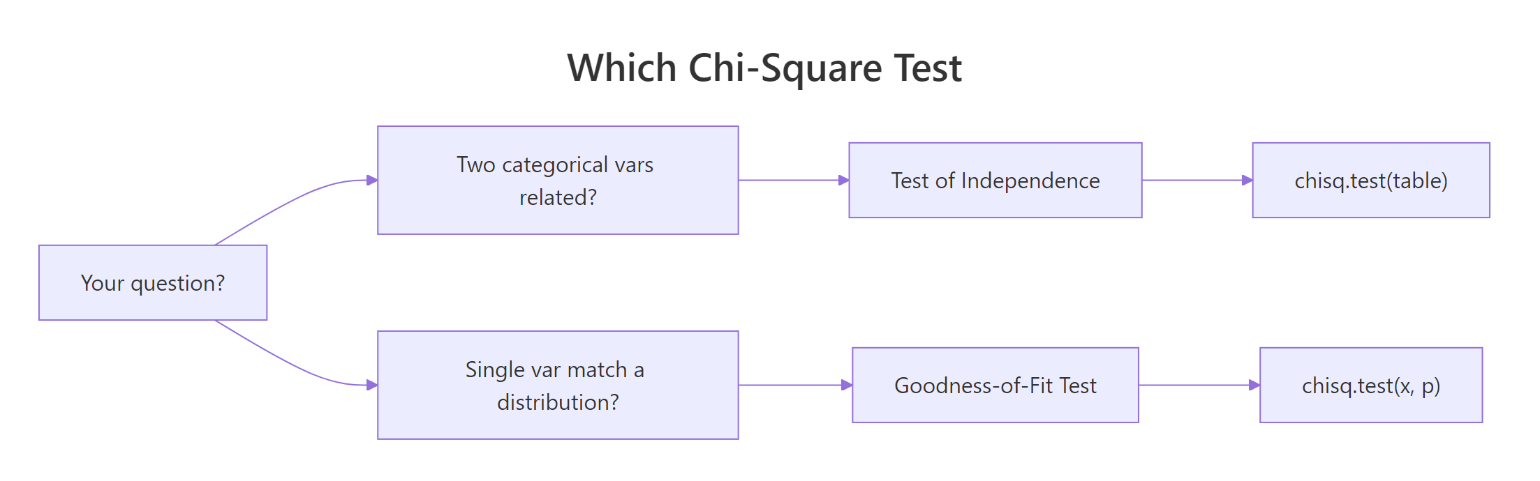
Choosing between the test of independence and goodness-of-fit.

Figure 1: Choosing between the test of independence and goodness-of-fit.

Most real data arrives as one row per observation, not as a pre-built table. You build the contingency table with table(), then pass it to chisq.test().

RBuild a contingency table and test independence

cyl_am <- table(mtcars$cyl, mtcars$am) cyl_am #> #> 0 1 #> 4 3 8 #> 6 4 3 #> 8 12 2 cyl_am_test <- chisq.test(cyl_am) cyl_am_test #> #> Pearson's Chi-squared test #> #> data: cyl_am #> X-squared = 8.7407, df = 2, p-value = 0.01265

With X-squared = 8.74, df = 2, and p = 0.013, we reject independence at the 5% level. In this garage, manual cars cluster in the 4-cylinder group while automatics dominate the 8-cylinder group.

The returned object carries a lot more than what print() displays. You can pull out observed counts, expected counts, the statistic, degrees of freedom, and the p-value individually.

RAccess pieces of the chisq.test result

cyl_am_test$observed #> #> 0 1 #> 4 3 8 #> 6 4 3 #> 8 12 2 round(cyl_am_test$expected, 2) #> #> 0 1 #> 4 6.53 4.47 #> 6 4.16 2.84 #> 8 8.31 5.69 cyl_am_test$statistic #> X-squared #> 8.740733 cyl_am_test$parameter #> df #> 2 cyl_am_test$p.value #> [1] 0.01265483

The $expected matrix shows what each cell would contain if cylinders and transmission were truly independent: roughly 6.5 manual 4-cylinders, not the 8 we actually observed. Bigger gaps between observed and expected mean a bigger chi-square.

Key Insight

The chi-square statistic is the squared standardized gap between observed and expected, summed across all cells. In symbols, $\chi^2 = \sum (O - E)^2 / E$. Each cell contributes a non-negative term; large contributions come from cells where observed counts are far from what independence predicts.

Try it: Build a table of mtcars$gear versus mtcars$am and test whether the two are independent.

RYour turn: gears vs transmission

# Try it: independence test of gear and am ex_gear_am <- # your code here chisq.test(ex_gear_am) #> Expected: A chi-square statistic and a very small p-value

Click to reveal solution

RGears vs transmission solution

ex_gear_am <- table(mtcars$gear, mtcars$am) chisq.test(ex_gear_am) #> #> Pearson's Chi-squared test #> #> data: ex_gear_am #> X-squared = 20.935, df = 2, p-value = 2.832e-05

Explanation: Gear count and transmission type are strongly related: 3- and 4-gear cars are mostly manual/automatic in opposite proportions, which shows up as a tiny p-value.

How do you run a chi-square goodness-of-fit test?

Goodness-of-fit flips the question. Instead of two variables, you have one variable and a claimed distribution. Does your observed count vector look like it came from that distribution? The function is the same, chisq.test(), but you pass the counts as x and the hypothesized probabilities as p.

The simplest case is "all categories equally likely." Suppose we rolled a die 152 times and saw the counts below. Is it a fair die?

RGoodness-of-fit for a fair die

die_rolls <- c(22, 19, 27, 32, 28, 24) die_test <- chisq.test(die_rolls) die_test #> #> Chi-squared test for given probabilities #> #> data: die_rolls #> X-squared = 3.9474, df = 5, p-value = 0.5569

With p = 0.56, we do not reject fairness. The observed counts wander around 152/6 ≈ 25.3, but not further than sampling noise would explain on 5 degrees of freedom (k - 1 for k = 6 categories).

Real hypotheses rarely say "equal." Classical genetics predicts Mendel's 9:3:3:1 ratio for a dihybrid cross. Pass the ratio as p, and R will normalise it for you if you set rescale.p = TRUE, or you can divide yourself.

RGoodness-of-fit for Mendel's 9:3:3:1 ratio

mendel_counts <- c(315, 108, 101, 32) mendel_test <- chisq.test(mendel_counts, p = c(9, 3, 3, 1) / 16) mendel_test #> #> Chi-squared test for given probabilities #> #> data: mendel_counts #> X-squared = 0.47002, df = 3, p-value = 0.9254

A p-value of 0.93 is famously high, and the data match the 9:3:3:1 prediction almost perfectly on 3 degrees of freedom (k - 1 for k = 4 categories).

Tip

Use rescale.p = TRUE when your p vector doesn't sum to 1. You can pass p = c(9, 3, 3, 1) with rescale.p = TRUE and skip the manual division. It's safer than hand-normalising when the ratio is long.

Try it: Human blood types in a reference population are roughly 45% O, 40% A, 11% B, 4% AB. You collect 500 donors with counts 230, 190, 60, 20. Test whether the sample matches the reference distribution.

RYour turn: blood-type goodness-of-fit

# Try it: goodness-of-fit for blood types ex_blood <- c(230, 190, 60, 20) ex_ref <- # fill in the reference probabilities chisq.test(x = ex_blood, p = ex_ref) #> Expected: A chi-square statistic, df = 3, and a p-value

Click to reveal solution

RBlood-type goodness-of-fit solution

ex_blood <- c(230, 190, 60, 20) ex_ref <- c(0.45, 0.40, 0.11, 0.04) chisq.test(x = ex_blood, p = ex_ref) #> #> Chi-squared test for given probabilities #> #> data: ex_blood #> X-squared = 1.4646, df = 3, p-value = 0.6905

Explanation: Pass the reference proportions to p. A p-value of 0.69 says the sample is consistent with the reference distribution.

What are the assumptions of the chi-square test?

Three assumptions hold the chi-square test together:

Independent observations. Each count comes from a separate, independent unit. Repeated measurements on the same subject break this.
Expected counts large enough. The usual rule is that every expected count should be ≥ 5, and no fewer than 80% of cells should be below 5. Below that, the chi-square approximation to the sampling distribution gets unreliable.
Fixed categories, random sampling. The categories are defined before data collection; within that frame, observations were sampled randomly.

The most common violation is number 2. You can check it directly from the test object.

RProgrammatic check of expected-count assumption

small_tbl <- matrix(c(2, 8, 3, 1), nrow = 2, dimnames = list(Treatment = c("A", "B"), Outcome = c("Success", "Failure"))) small_tbl #> Outcome #> Treatment Success Failure #> A 2 3 #> B 8 1 small_test <- suppressWarnings(chisq.test(small_tbl)) round(small_test$expected, 2) #> Outcome #> Treatment Success Failure #> A 3.57 1.43 #> B 6.43 2.57 all(small_test$expected >= 5) #> [1] FALSE mean(small_test$expected >= 5) #> [1] 0

Every expected count is below 5, so the chi-square p-value for this table should not be trusted. R itself flags this with the message "Chi-squared approximation may be incorrect" when you call chisq.test() without suppressWarnings().

Warning

"Chi-squared approximation may be incorrect" is not decorative. When R prints this warning, at least one expected count is below 5 and the p-value is suspect. Use Fisher's exact test or the Monte-Carlo option (covered later) instead of ignoring the warning.

Try it: Given the 2×3 table below, check whether every expected count is ≥ 5.

RYour turn: check expected counts

# Try it: check the expected-counts rule on ex_mat ex_mat <- matrix(c(10, 15, 20, 12, 18, 25), nrow = 2, byrow = TRUE) ex_test <- suppressWarnings(chisq.test(ex_mat)) # your code here: check whether min(expected) is >= 5 #> Expected: TRUE (all expected counts pass the rule)

Click to reveal solution

RCheck expected counts solution

ex_mat <- matrix(c(10, 15, 20, 12, 18, 25), nrow = 2, byrow = TRUE) ex_test <- suppressWarnings(chisq.test(ex_mat)) all(ex_test$expected >= 5) #> [1] TRUE

Explanation: all(ex_test$expected >= 5) returns a single TRUE if every cell clears the threshold.

How do you interpret Pearson residuals?

A significant chi-square tells you something is off, but not where. Pearson residuals fix that. Each cell's residual is its standardized gap between observed and expected: positive when the cell has more observations than independence predicts, negative when it has fewer.

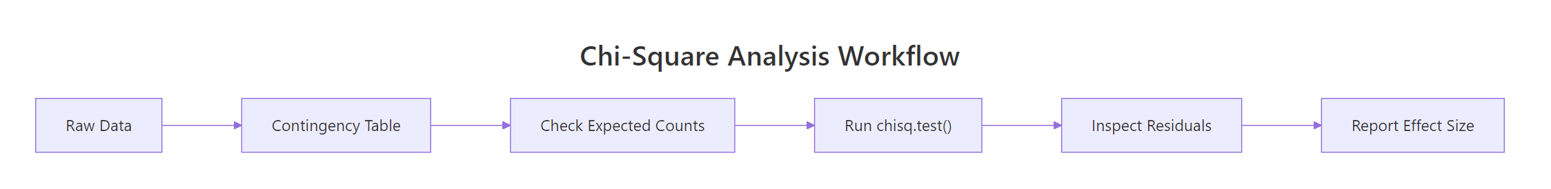
Standard workflow for a chi-square analysis.

Figure 2: Standard workflow for a chi-square analysis.

R gives you two residual matrices:

$residuals: Pearson residuals, $(O - E) / \sqrt{E}$. Useful for the $statistic math but not directly calibrated.
$stdres: standardized residuals, rescaled to approximately a standard normal. Cells with |stdres| > 2 are roughly at p < 0.05 locally.

RPearson and standardized residuals for hair-eye

round(he_test$residuals, 2) #> Eye #> Hair Brown Blue Hazel Green #> Black 4.40 -3.07 -0.48 -1.95 #> Brown 1.23 -1.95 1.35 -0.35 #> Red -0.07 -1.73 0.85 2.28 #> Blond -5.85 7.05 -2.23 0.61 round(he_test$stdres, 2) #> Eye #> Hair Brown Blue Hazel Green #> Black 5.80 -3.97 -0.56 -2.27 #> Brown 2.20 -3.39 2.05 -0.46 #> Red -0.07 -1.95 0.89 2.36 #> Blond -7.34 8.60 -2.60 0.68

The biggest positive residual is Blond × Blue at 8.6, the biggest negative is Blond × Brown at −7.3. In plain language: blond people are massively over-represented among blue-eyed subjects and under-represented among brown-eyed subjects, which is what drives the huge chi-square we saw in block 1.

A tile plot makes this visible at a glance. We convert the standardized residuals to a long data frame, then let ggplot colour them red-to-blue.

RTile plot of standardized residuals

res_df <- as.data.frame(as.table(he_test$stdres)) names(res_df) <- c("Hair", "Eye", "stdres") ggplot(res_df, aes(Eye, Hair, fill = stdres)) + geom_tile(colour = "white") + geom_text(aes(label = round(stdres, 1)), size = 4) + scale_fill_gradient2(low = "#2166AC", mid = "white", high = "#B2182B", midpoint = 0) + labs(title = "Hair vs Eye colour: standardized residuals", fill = "stdres") + theme_minimal()

Red cells flag categories that are over-represented; blue cells flag under-representation. This is the single most useful follow-up graphic after any significant test of independence.

Tip

A rule of thumb: |stdres| > 2 marks a cell worth writing about. Under the null of independence, standardized residuals are approximately standard normal, so values beyond ±2 correspond roughly to local p < 0.05. For strict inference across many cells, apply a Bonferroni correction.

Try it: Using he_test, find the two cells with the largest absolute standardized residual.

RYour turn: find the top-2 residual cells

# Try it: identify the two largest |stdres| cells ex_res <- he_test$stdres # your code here: return the two cells with largest absolute values #> Expected: Blond-Brown (~-7.3) and Blond-Blue (~8.6)

Click to reveal solution

RTop-2 residual cells solution

ex_res <- he_test$stdres ex_sorted <- sort(abs(ex_res), decreasing = TRUE) head(ex_sorted, 2) #> [1] 8.596 7.344

Explanation: Flatten the matrix with sort() on its absolute values; the top two entries correspond to the Blond × Blue and Blond × Brown cells.

How do you measure effect size with Cramér's V?

A p-value answers "is there a relationship?" It does not answer "how strong?" With enough data, even a trivial association can look statistically significant. Effect size fixes that.

For a test of independence, the standard effect size is Cramér's V:

$$V = \sqrt{\frac{\chi^2}{n \cdot \min(r - 1,\ c - 1)}}$$

Where:

$\chi^2$ is the test statistic from chisq.test()
$n$ is the total sample size
$r$ and $c$ are the numbers of rows and columns in the table

V ranges from 0 (no association) to 1 (perfect association). Cohen's conventions call V ≈ 0.1 small, 0.3 medium, and 0.5 large, but always calibrate against your own field.

For goodness-of-fit, the equivalent is Cohen's w:

$$w = \sqrt{\frac{\chi^2}{n}}$$

where $n$ is again the total count. Same small/medium/large conventions.

RCompute Cramer's V and Cohen's w

cramers_v <- function(test_result) { chi2 <- test_result$statistic n <- sum(test_result$observed) k <- min(nrow(test_result$observed), ncol(test_result$observed)) sqrt(chi2 / (n * (k - 1))) } cohens_w <- function(test_result) { sqrt(test_result$statistic / sum(test_result$observed)) } unname(cramers_v(he_test)) #> [1] 0.2791 unname(cohens_w(mendel_test)) #> [1] 0.02427

Hair and eye colour show a medium-sized association (V ≈ 0.28), strong enough to be practically meaningful and not just statistically significant. The Mendel cross gives an effect size of essentially 0, confirming that observed counts line up tightly with the 9:3:3:1 prediction.

Key Insight

Cramér's V strips out sample size, so it's comparable across studies. Two researchers can run the same question on samples of 100 and 10,000 and report V values you can legitimately compare; raw chi-square values, which scale with n, cannot be.

Try it: Compute Cramér's V for the cylinders × transmission result cyl_am_test from an earlier section.

RYour turn: Cramer's V for cyl vs am

# Try it: compute Cramer's V for cyl_am_test ex_v <- # your code here ex_v #> Expected: approximately 0.52 (a large effect)

Click to reveal solution

RCramer's V for cyl vs am solution

ex_v <- cramers_v(cyl_am_test) unname(ex_v) #> [1] 0.5227

Explanation: The function we defined works on any chisq.test() result. V = 0.52 flags a large effect, even though the table is small.

When should you use Fisher's exact test instead?

When expected counts are small, the chi-square approximation breaks down. Two robust alternatives live in base R:

Fisher's exact test (fisher.test()): uses the exact hypergeometric distribution, so no approximation is needed. Designed for 2×2 tables; also works on larger tables at higher computational cost.
Monte-Carlo p-value (chisq.test(..., simulate.p.value = TRUE, B = 10000)): simulates B tables under the null and reports the proportion with a statistic at least as extreme as yours. Works on any table.

Here's a 2×2 with small counts where the plain chi-square warning fires, compared against both alternatives.

RFisher vs chi-square vs Monte Carlo on small 2x2

tiny_tbl <- matrix(c(2, 8, 9, 3), nrow = 2, dimnames = list(Drug = c("A", "B"), Outcome = c("Cure", "No cure"))) tiny_tbl #> Outcome #> Drug Cure No cure #> A 2 9 #> B 8 3 suppressWarnings(chisq.test(tiny_tbl))$p.value #> [1] 0.02062 fisher.test(tiny_tbl)$p.value #> [1] 0.03008 set.seed(2026) chisq.test(tiny_tbl, simulate.p.value = TRUE, B = 10000)$p.value #> [1] 0.03

All three agree that drugs A and B differ, but the plain chi-square reports the smallest p-value (0.021) because the approximation is pushed too hard. Fisher's exact (0.030) and Monte Carlo (0.030) agree and are trustworthy on this sample size.

Tip

simulate.p.value = TRUE is the general-purpose escape hatch. It works on any size table, returns a valid p-value even when expected counts are below 5, and is built into chisq.test() itself. Set B to 10,000 or more for a stable estimate.

Try it: Run Fisher's exact test on the 2×2 below, and report the p-value.

RYour turn: run Fisher's exact test

# Try it: Fisher's exact on ex_small ex_small <- matrix(c(3, 7, 10, 2), nrow = 2) # your code here #> Expected: a p-value around 0.02

Click to reveal solution

RFisher's exact solution

ex_small <- matrix(c(3, 7, 10, 2), nrow = 2) fisher.test(ex_small)$p.value #> [1] 0.01984

Explanation: fisher.test() accepts the matrix directly and returns a result whose $p.value is the exact hypergeometric p-value.

Practice Exercises

Exercise 1: Admissions at Berkeley

Use the UCBAdmissions dataset (built-in 3D array: Admit × Gender × Dept). Collapse over department with margin.table(UCBAdmissions, c(1, 2)) to get a 2×2 table of admission × gender. Run a chi-square test of independence, compute Cramér's V using the helper defined earlier, and write a one-sentence conclusion.

RExercise 1: UCB admissions

# Exercise: test independence of admission and gender; report V # Hint: use margin.table() then cramers_v() my_ucb <- # build the 2-way table # Write your code below:

Click to reveal solution

RUCB admissions solution

my_ucb <- margin.table(UCBAdmissions, c(1, 2)) my_ucb #> Gender #> Admit Male Female #> Admitted 1198 557 #> Rejected 1493 1278 my_ucb_test <- chisq.test(my_ucb) my_ucb_test$statistic #> X-squared #> 91.6096 my_ucb_test$p.value #> [1] 1.055e-21 unname(cramers_v(my_ucb_test)) #> [1] 0.1439

Explanation: The naïve analysis shows a highly significant association (p < 10⁻²⁰) with a small-to-medium effect (V ≈ 0.14), suggesting gender bias in admissions. This is the famous Simpson's paradox setup: stratifying by department reverses the story, which is why always stratifying before aggregating is a cardinal rule of categorical analysis.

Exercise 2: Detect a loaded die

Simulate 200 rolls from a six-sided die with unequal probabilities (face 6 boosted), then run a goodness-of-fit test against the fair-die hypothesis and report Cohen's w.

RExercise 2: detect a loaded die

# Exercise: simulate loaded die, test fairness, report Cohen's w # Hint: use sample() with a custom prob vector, then table() set.seed(2026) my_probs <- c(0.15, 0.15, 0.15, 0.15, 0.15, 0.25) # Write your code below:

Click to reveal solution

RLoaded die solution

set.seed(2026) my_probs <- c(0.15, 0.15, 0.15, 0.15, 0.15, 0.25) my_rolls <- sample(1:6, 200, replace = TRUE, prob = my_probs) my_counts <- as.numeric(table(factor(my_rolls, levels = 1:6))) my_counts #> [1] 30 23 24 36 28 59 my_gof <- chisq.test(my_counts) my_gof #> #> Chi-squared test for given probabilities #> #> data: my_counts #> X-squared = 24.62, df = 5, p-value = 0.0001662 unname(cohens_w(my_gof)) #> [1] 0.3509

Explanation: The test rejects fairness with p < 0.001, and Cohen's w ≈ 0.35 flags a medium-to-large effect, consistent with the deliberate boost on face 6.

Exercise 3: Small-sample decision

The 2×2 table below shows treatment success in a very small pilot trial. Decide between chisq.test(), chisq.test(..., simulate.p.value = TRUE), and fisher.test(). Justify your pick, then run it.

RExercise 3: small-sample decision

# Exercise: pick the right test for this 2x2 my_pilot <- matrix(c(1, 9, 7, 3), nrow = 2, dimnames = list(Arm = c("New", "Control"), Outcome = c("Success", "Failure"))) my_pilot # Write your code below (and comment your justification):

Click to reveal solution

RSmall-sample decision solution

my_pilot <- matrix(c(1, 9, 7, 3), nrow = 2, dimnames = list(Arm = c("New", "Control"), Outcome = c("Success", "Failure"))) my_exp <- suppressWarnings(chisq.test(my_pilot))$expected round(my_exp, 2) #> Outcome #> Arm Success Failure #> New 4.00 6.00 #> Control 4.00 6.00 all(my_exp >= 5) #> [1] FALSE fisher.test(my_pilot) #> #> Fisher's Exact Test for Count Data #> #> p-value = 0.01963 #> alternative hypothesis: true odds ratio is not equal to 1

Explanation: Two of the four expected counts fall below 5, so the chi-square approximation is unreliable. Fisher's exact test is the textbook choice for a small 2×2 and reports p = 0.020, flagging a significant difference between arms.

Complete Example

Let's tie every step together on the Titanic dataset: collapse over Age and Class to get a 2-way Sex × Survived table, then run the full workflow: assumption check, chi-square, residuals, effect size, interpretation.

RComplete example: Titanic survival by sex

titanic_2d <- margin.table(Titanic, c(2, 4)) titanic_2d #> Survived #> Sex No Yes #> Male 1364 367 #> Female 126 344 tit_test <- chisq.test(titanic_2d) round(tit_test$expected, 0) #> Survived #> Sex No Yes #> Male 1175 556 #> Female 319 151 all(tit_test$expected >= 5) #> [1] TRUE tit_test #> #> Pearson's Chi-squared test with Yates' continuity correction #> #> data: titanic_2d #> X-squared = 454.5, df = 1, p-value < 2.2e-16 round(tit_test$stdres, 2) #> Survived #> Sex No Yes #> Male 21.6 -21.6 #> Female -21.6 21.6 tit_v <- unname(cramers_v(tit_test)) tit_v #> [1] 0.4891

How to read it. Expected counts all clear the ≥ 5 rule, so the chi-square p-value is trustworthy. The test rejects independence overwhelmingly (X² = 454, p < 10⁻¹⁵). Standardized residuals show males massively under-represented among survivors and females massively over-represented. Cramér's V ≈ 0.49 is a near-large effect, quantifying exactly how strong the "women first" pattern was on the Titanic.

Summary

Question	R function	df formula	Effect size
Are two categorical variables related?	`chisq.test(table(x, y))`	(r - 1)(c - 1)	Cramér's V
Does one variable match a distribution?	`chisq.test(x, p = probs)`	k - 1	Cohen's w
Small expected counts?	`fisher.test()` or `simulate.p.value = TRUE`	N/A	N/A
Which cells drive the result?	`result$stdres` (	value	> 2)	N/A	N/A

Key takeaways:

Pass raw counts, never proportions.
Check $expected ≥ 5 before trusting the p-value.
Always report an effect size, Cramér's V for independence or Cohen's w for goodness-of-fit.
Inspect residuals to explain where the association lives.
Switch to Fisher's exact or Monte Carlo when the approximation warning fires.

Chi-square tests at a glance.

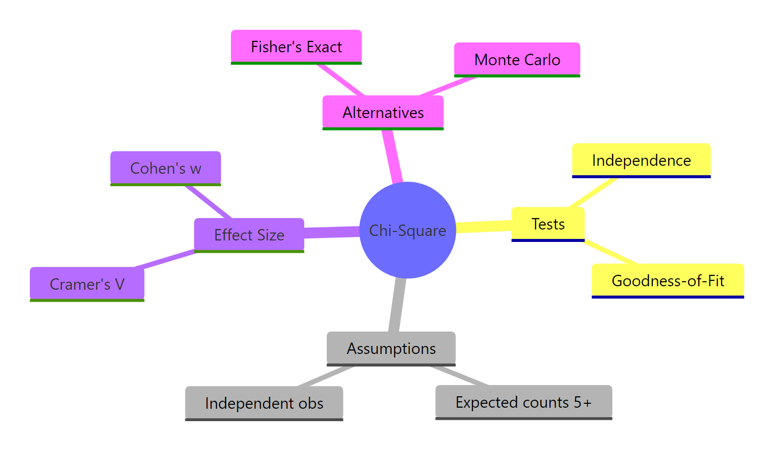
Figure 3: Chi-square tests at a glance.

References

R Core Team. stats::chisq.test documentation. Link
Agresti, A. Categorical Data Analysis, 3rd ed. Wiley (2013).
Cohen, J. Statistical Power Analysis for the Behavioral Sciences, 2nd ed. Lawrence Erlbaum (1988).
Cramér, H. Mathematical Methods of Statistics. Princeton University Press (1946).
Sharpe, D. "Your Chi-Square Test is Statistically Significant: Now What?" Practical Assessment, Research & Evaluation, 20(8), 2015. Link
Fisher, R.A. Statistical Methods for Research Workers. Oliver & Boyd (1925).
Kim, H.-Y. "Statistical notes for clinical researchers: Chi-squared test and Fisher's exact test." Restorative Dentistry & Endodontics, 42(2), 2017. Link
Agresti, A. An Introduction to Categorical Data Analysis, 3rd ed. Wiley (2018).

Continue Learning

Hypothesis Testing in R: the inference framework chi-square sits inside.
t-Tests in R: the chi-square equivalent for comparing means of numeric groups.
Proportion Tests in R: an alternative when your question is about a single proportion or difference of proportions.

Chi-Square Tests in R: Independence, Goodness-of-Fit, With Effect Sizes

When should you use a chi-square test?

How do you run a chi-square test of independence?

How do you run a chi-square goodness-of-fit test?

What are the assumptions of the chi-square test?

How do you interpret Pearson residuals?

How do you measure effect size with Cramér's V?

When should you use Fisher's exact test instead?

Practice Exercises

Exercise 1: Admissions at Berkeley

Exercise 2: Detect a loaded die

Exercise 3: Small-sample decision

Complete Example

Summary

References

Continue Learning

Related Tutorials