Functional Programming in R: The Mindset That Makes Your Code 10× Cleaner

Functional programming in R is the discipline of treating functions as ordinary values, you can store them, pass them around, and compose them, so repetitive loops collapse into single lines that say exactly what they do. Once the mindset clicks, most of your R code gets dramatically shorter, safer, and easier to read.

Why is functional programming a mindset, not a package?

You've written the loop before: declare an empty vector, count indices, assign by position, try not to break the bookkeeping. It works, but most of the code is scaffolding, not meaning. Functional style flips that ratio. You describe the transformation once and hand it to R, the iteration disappears into a single call. Here is the same answer, both ways.

Both blocks produce the same vector. The loop spends four lines managing an index and a result buffer before it ever mentions squaring. The sapply call says, in one line, "apply this function to each element." That is the entire pitch of functional style: stop writing the bookkeeping, start writing the meaning.

How are functions first-class objects in R?

"First-class" is a claim about status: a value is first-class when you can do the same things to it that you can do to any other value. Integers are first-class, you can assign them, put them in a list, pass them to a function, or return them. In R, functions have exactly the same privileges. Seeing the proof of that is the fastest way to unlock the mindset.

double is now a name that refers to a function, exactly the way x <- 7 makes x refer to a number. The ops list holds three functions together, each retrievable with $. If this feels normal, good, that is the goal. Functions in R are ordinary values you can carry around in any container.

The other two privileges are "pass as an argument" and "return from another function." Here is a function that takes another function and applies it twice.

apply_twice is a higher-order function: a function whose argument (or return value) is itself a function. The first call hands over double, the second hands over an inline anonymous function. R treats them identically because, to R, they are just values of type function.

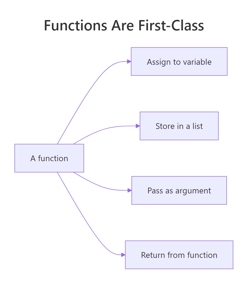
Figure 1: Four things you can do with a function that you can also do with any value.

What are map, filter, and reduce, R's three core functionals?

Nearly every repetitive task on a collection fits one of three shapes. Map transforms each element, filter keeps elements that pass a test, and reduce collapses everything into a single value. R ships all three as base functions, Map(), Filter(), and Reduce(), plus the friendly vector-returning cousins sapply() and vapply(). Once you recognise the three shapes, you will spot them everywhere.

Read from top to bottom: Map returned a list (one squared value per input), sapply did the same job but gave back a plain numeric vector, Filter kept only the even values, and Reduce collapsed 1:6 to the sum 21. The accumulate = TRUE variant is a debugging gift, it shows you every intermediate value, so you can see why repeatedly adding 1:6 must end at 21.

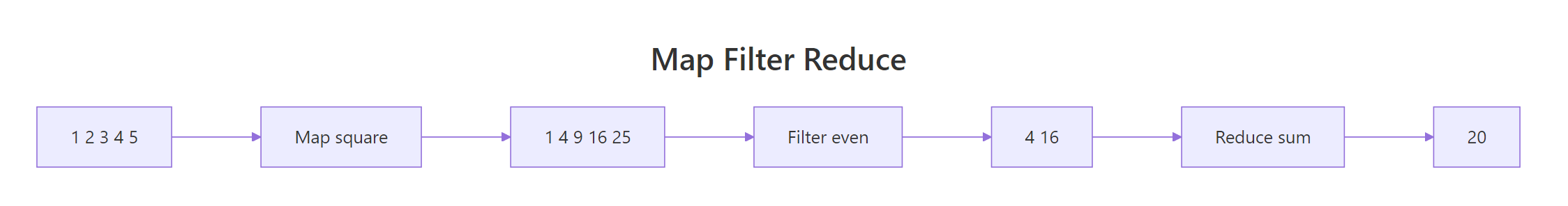
Figure 2: How map, filter, and reduce transform a collection step by step.

How do pure functions and closures power functional style?

Two ideas make functional code safe and reusable. A pure function depends only on its arguments and changes nothing else, given the same inputs, it always returns the same output. A closure is a function that remembers the environment it was created in, so it can carry a piece of state without using a global variable. Together they explain why functional R is easy to test and easy to compose.

add(2, 3) will return 5 forever, no matter how many times or in what order you call it, that is purity. impure_increment() returns a different number on every call because its answer depends on the hidden counter variable. Impure functions can be useful, but they make code harder to reason about: to predict the output, you need to know the history of every prior call. Functional style prefers purity because purity is what makes Map, Filter, and Reduce trustworthy, R can call them in any order without surprises.

A closure looks similar but uses the outer environment in a controlled, read-only way.

make_multiplier(3) returns a brand-new function whose body refers to factor. That factor lives in the environment make_multiplier was running in when it returned, and the returned function keeps a reference to it forever. times_three and times_ten are two different closures, each remembering its own factor. This is how you build specialised functions from a general recipe, no classes, no templates, just one line.

When should you reach for functional style instead of a loop?

Not every loop needs to be refactored. If the loop is tiny, imperative, and easier to read than the alternative, leave it alone, the goal is clarity, not ideological purity. But the moment a loop is describing a transformation (each → something), a filter (keep items where), or an accumulation (combine all into one), that loop is secretly a functional, and rewriting it usually shrinks the code by half.

Here is a concrete comparison on the built-in mtcars dataset, compute the mean of three columns.

Both versions return the same named numeric vector. The functional version is a single line because sapply already knows how to iterate over a list (a data frame is a list of columns) and collect results by name. The loop version needs four lines to reproduce that plumbing by hand. Read the sapply line aloud: "apply mean to each of these columns." That sentence is the code.

If you work in the tidyverse, the same idea is one line of purrr:

map_dbl is the type-stable sibling of sapply: it returns a double vector or it errors, it never silently gives you a list. That guarantee is the main reason purrr exists alongside base R's functionals.

A practical decision list:

1. Describing a transformation? Use sapply, Map, or purrr::map_*.
2. Keeping only some elements? Use Filter or purrr::keep.
3. Collapsing to one value? Use Reduce or purrr::reduce.
4. Need a running side-effect like printing, plotting, or writing files? Use for, or purrr::walk if you want the functional style, side effects are legal, they are just not the functionals' strength.

Practice Exercises

These capstones combine two or more ideas from the tutorial. Each uses distinct variable names prefixed with my_ so you can experiment without overwriting tutorial state.

Exercise 1: Filter then map for word lengths

Given the list below, use Filter and sapply together to return a numeric vector of lengths of words that have at least 5 letters. Save the result to my_long_lengths.

Exercise 2: Build a power function with a factory

Write a function factory make_power(n) that returns a function raising its input to the nth power. Use it to create cube and then apply cube to 1:5. Save the resulting vector to my_cubes.

Exercise 3: Running factorial with accumulate

Use Reduce with accumulate = TRUE to compute the running product of 1:6, these are the factorials 1!, 2!, 3!, up to 6!. Save the resulting vector to my_factorials.

Complete Example

Let's put all five ideas to work on a tiny but realistic task: given a small inventory, compute the average price of items that are currently in stock. This example uses first-class functions (stored in a list-of-records), a filter, a map, and a reduce, the whole FP toolkit on three lines of data.

Each step has a single job and a single shape. You filter to drop out-of-stock items, map to extract the field you care about, and reduce to collapse many values into one. Every intermediate result is visible, so debugging is trivial, you check each pipe one at a time. Once the steps work, you can chain them into a single line for production:

That one-liner is the reward for learning the vocabulary. It reads right to left like a sentence: "take the mean of the prices of the in-stock items in inventory." Your future self will thank you for writing it this way.

Summary

Functional programming in R is a mindset before it is a toolkit. Once you accept that functions are ordinary values, the rest falls out naturally, map, filter, and reduce become the obvious way to describe repetitive work, pure functions become the obvious way to keep results predictable, and closures become the obvious way to build specialised workers from a single recipe.

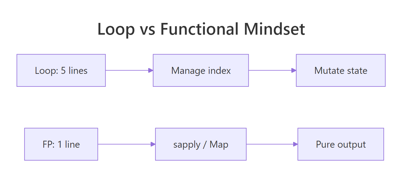
Figure 3: The mental move from looping to functional style.

Five takeaways to keep:

1. Functions are values. Assign them, store them in lists, pass them as arguments, return them from other functions.
2. Three shapes cover most iteration. Transform with Map/sapply, filter with Filter, collapse with Reduce. Spot the shape, pick the functional.
3. Pure functions are easier to reason about. Same inputs, same output, no hidden state, that is the guarantee that makes composition safe.
4. Closures carry state cleanly. A function returned from another function remembers the environment it was born in, use that to build specialised workers.
5. Start with base R, graduate to purrr. sapply, Map, Filter, Reduce teach the vocabulary. purrr::map_dbl and friends add type safety when you need it.

References

1. Wickham, H., Advanced R, 2nd Edition. Chapter 9: Functionals. Link
2. Wickham, H., Advanced R, 2nd Edition. Chapter 6: Functions. Link
3. Peng, R. D., Mastering Software Development in R, §2.3 Functional Programming. Link
4. R Core Team, Map, Filter, Reduce reference (funprog). Link
5. purrr tidyverse package documentation. Link
6. Rodrigues, B., Modern R with the tidyverse, Chapter 8: Functional Programming. Link

Continue Learning

• purrr map() Variants, the type-stable, pipe-friendly modern alternative to sapply.
• R Anonymous Functions, a deep dive into function(x) ... and the R 4.1+ shorthand \(x) ....
• Reduce, Filter, Map in R, a focused walkthrough of the base-R trio with more examples.