Multinomial & Ordinal Logistic Regression in R: Beyond Binary Outcomes
Binary logistic regression covers two-outcome problems. When your response has three or more categories, you need multinomial (unordered) or ordinal (ordered) logistic regression. This tutorial shows how to fit, interpret, and predict with both, using nnet::multinom() and MASS::polr() on built-in R datasets so every block runs end-to-end.
What's the difference between binary, multinomial, and ordinal logistic regression?
Binary logistic regression handles exactly two outcomes: yes or no, click or skip, churn or stay. Real datasets often offer more options. The iris dataset has three species. A satisfaction survey can rank low, medium, or high. The right model depends on whether your categories are simply different (multinomial) or ranked from low to high (ordinal). Let's see the payoff first by predicting iris species with one short multinomial fit, then take it apart piece by piece.
In nine lines we fit a model with three outcome classes and got back a row of class probabilities for every flower. The first three iris rows are all setosa, and the model assigns near-1 probability to setosa for each. That is the multinomial logistic regression workflow at a glance. The next sections explain how the function decides those numbers and how to extend the same idea when categories are ranked.
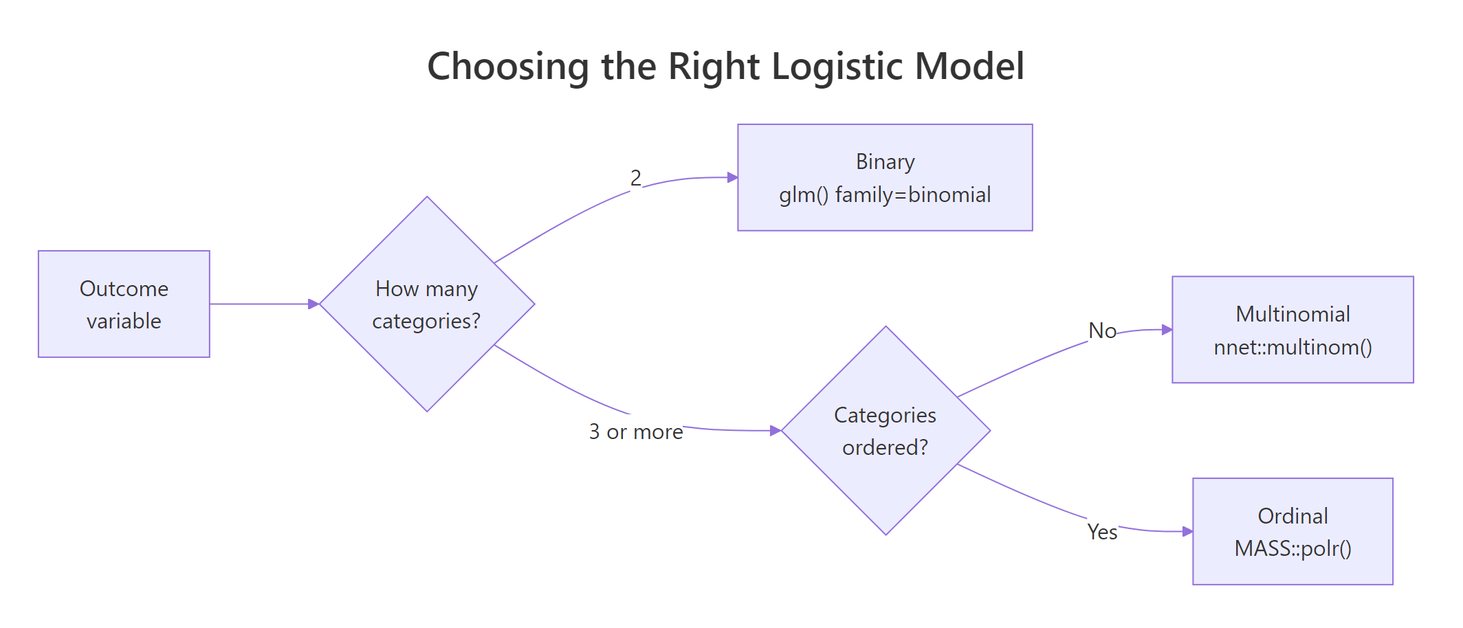
Figure 1: Choosing among binary, multinomial, and ordinal logistic regression by counting categories and asking whether they are ordered.
The decision tree is short. Two outcomes go to plain glm(family = binomial). Three or more unordered categories (species, brand chosen, disease subtype) go to multinomial. Three or more ordered categories (low / medium / high satisfaction, star ratings, disease severity) go to ordinal. Picking the wrong one costs you either accuracy or interpretability.
Try it: Predict the probability vector for an "average" iris flower with Sepal.Length = 6 and Petal.Length = 4. Round the result to three decimals.
Click to reveal solution
Explanation: With moderate sepal length and a petal of 4cm, the model leans heavily toward versicolor and gives setosa essentially zero. Probabilities always sum to 1.
How do you fit a multinomial logistic regression with multinom()?
The workhorse is nnet::multinom(). It takes the same formula syntax as lm() or glm(), picks the first level of the response factor as the reference, and fits one set of coefficients for each remaining class. There is no family = argument because the model class is fixed.
The coefficient table has two rows because iris has three species and setosa (alphabetically first) is the reference. The first row maps setosa -> versicolor, the second row maps setosa -> virginica. Each column reads as: how a one-unit change in that predictor shifts the log relative-risk of being in that class versus the reference, holding the other predictors fixed. The signs already tell a story: Petal.Length is a strong positive driver of both non-setosa classes, which matches the well-known pattern that setosa has small petals.
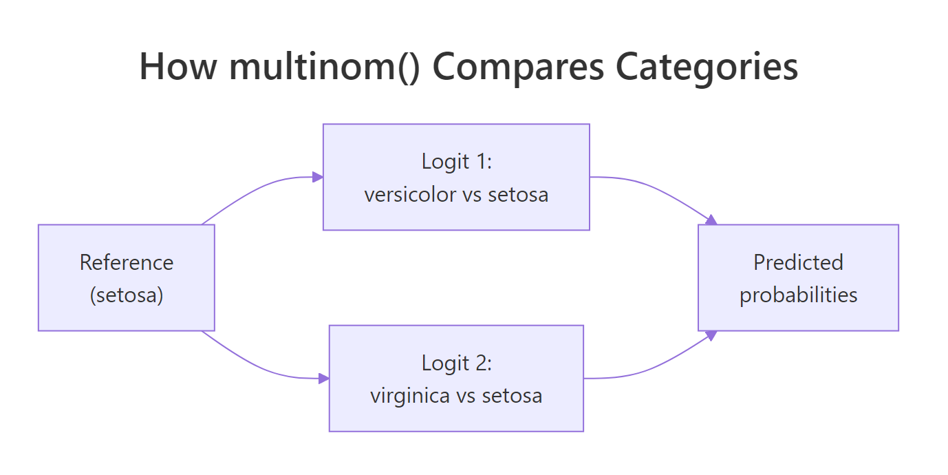
Figure 2: multinom() splits a K-class problem into K-1 binary logits against a single reference category.
You don't have to live with the alphabetical reference. Use relevel() to pin whichever class is your natural baseline. Below we make versicolor the reference and refit, and the coefficient rows now describe versicolor -> setosa and versicolor -> virginica.
Switching the reference does not change the model, only how you read it. The likelihoods, predicted probabilities, and AIC all stay the same. What flips is the comparison baseline for every coefficient. Choose the reference that makes your write-up easiest to read.
Try it: Make virginica the reference category and fit a model with Petal.Length only. How many coefficient rows should you see?
Click to reveal solution
Explanation: A K-class outcome always produces K-1 coefficient rows. With 3 species and virginica as reference, you get rows for setosa and versicolor.
How do you interpret multinomial coefficients and odds ratios?
Coefficients on the log scale are hard to read. Exponentiate them and you get relative risk ratios (often called odds ratios in the multinomial setting). A value above 1 means the predictor pushes flowers toward that class versus the reference; a value below 1 pushes them away. Exponentiation also handles the second log step in this formula:
$$\log \frac{P(Y=k)}{P(Y=\text{ref})} = \beta_{0k} + \beta_{1k}x_1 + \dots + \beta_{pk}x_p$$
Where:
- $P(Y=k)$ is the probability of class $k$
- $P(Y=\text{ref})$ is the probability of the reference class
- $\beta_{jk}$ is the coefficient for predictor $j$ in the equation for class $k$
- $x_j$ is the value of predictor $j$ for one observation
Read one row at a time. The Petal.Length column says that, holding the other variables fixed, a one-centimetre increase multiplies the relative risk of being virginica (vs setosa) by about $1.86 \times 10^{10}$. The number is huge because petal length is the single most discriminating feature in iris, not because the model is broken. The same predictor for versicolor vs setosa is also large but smaller, and Petal.Width swings strongly the other way: a wider petal pushes flowers toward virginica and away from versicolor.
Try it: Compute the relative risk ratio of Petal.Length for versicolor vs setosa from the original mfit and round it to one decimal.
Click to reveal solution
Explanation: A unit jump in petal length multiplies the odds of versicolor (vs setosa) by roughly 1.5 million. Big numbers reflect a near-deterministic split, not a bug.
How do you compute p-values, predictions, and a confusion matrix?
nnet::multinom() does not print p-values by default. The standard fix is a Wald z-test: divide each coefficient by its standard error, then compare to a normal distribution. The same fitted model also gives you predicted classes, predicted probabilities, and a confusion matrix in three short calls.
The matrix mirrors the coefficient layout: one row per non-reference class, one column per predictor. Most cells are well below 0.05, so the predictors carry real signal. The exception is Petal.Width for versicolor (p = 0.42), which suggests it adds little once the other variables are in the model. You would normally drop or test that predictor with a likelihood-ratio test before reporting.
type = "class" returns the highest-probability label per row, while type = "probs" returns the full probability matrix. Side by side, you can sanity-check the model: a high-confidence row means the model is decisive, while probabilities like 0.45 / 0.40 / 0.15 flag rows the model finds genuinely ambiguous.
The diagonal counts the correct calls. iris is famously easy: only two of 150 flowers are misclassified, both crossing the versicolor / virginica boundary. Accuracy works out to 98.7%, but remember that this is training accuracy, computed on the same rows the model was fit on.
Try it: Calculate accuracy from the confusion matrix without using diag(). Hint: extract the diagonal yourself.
Click to reveal solution
Explanation: Manually summing the diagonal makes the formula obvious: correct calls divided by all calls. diag() is the shortcut, not the definition.
How do you fit an ordinal logistic regression with polr()?
Switch to ordered categories and the toolkit changes. MASS::polr() fits a proportional odds logistic regression. Instead of K-1 separate intercepts and K-1 separate slopes, it shares one slope vector across all category boundaries and only the intercepts (the cut points) differ. The model is captured by:
$$\text{logit}\bigl(P(Y \le j \mid x)\bigr) = \alpha_j - \beta'x \quad \text{for } j = 1, \dots, J-1$$
Where:
- $P(Y \le j \mid x)$ is the cumulative probability of being at or below category $j$
- $\alpha_j$ is the cut point for boundary $j$ (there are $J-1$ of them)
- $\beta$ is the shared slope vector
- $x$ is the predictor vector
The built-in MASS::housing dataset has tenant satisfaction (Sat) coded as Low / Medium / High, plus weights (Freq) for each cell. That is exactly the ordered structure polr() expects.
Sat arrives as an ordered factor, which is what polr() requires. Hess = TRUE saves the Hessian so summary() can compute standard errors. The weights = Freq argument tells the fit that each row represents many tenants, not just one. Forgetting either argument is a common ordinal-regression bug.
ordered(x, levels = c("Low", "Medium", "High")) before fitting. If you forget, polr() will refuse the call or, worse, silently treat the levels in the wrong order.The first six rows are slopes (one per non-reference predictor level) and the last two are cut points. Reading InflHigh = 1.29 on the log scale or 3.63 after exponentiating: tenants with high perceived influence have 3.63 times the odds of being in a higher satisfaction category, compared with the low-influence reference. TypeTerrace = 0.34 says terrace tenants are about a third as likely to land in a higher satisfaction category as tower tenants.
Try it: Refit the ordinal model with Type as the only predictor and print its AIC. Is it lower or higher than the full model's AIC?
Click to reveal solution
Explanation: Dropping Infl and Cont raises AIC by about 190 points, confirming both predictors carry real explanatory power. Lower AIC is better.
How do you check the proportional odds assumption?
Ordinal models are simpler than multinomial models because they share one slope per predictor across all cut points. The price is an assumption: that single shared slope must actually fit the data. If it doesn't, predictions and standard errors get unreliable. Two cheap diagnostics catch most violations.
The first is to compare AIC against a multinomial fit on the same data. If the unconstrained multinom() is dramatically better, the parallel-lines constraint is hurting you. The second is the Brant test (brant::brant() in local R, which performs a chi-square per predictor).
The two AICs are almost identical (the ordinal model is even slightly lower). The penalty for sharing slopes across cut points buys you parsimony without giving up fit. That's a good sign that the proportional odds assumption holds for this dataset, and you can confidently report the ordinal model.
vglm() from VGAM with cumulative(parallel = FALSE ~ predictor)) or to reframe the response as multinomial.brant in a local R session and run brant::brant(ofit) to get one chi-square statistic per predictor plus an overall test. The closer the p-values are to 1, the safer the assumption.Try it: Compute the AIC difference (multinomial minus ordinal) for the housing fit and round to one decimal.
Click to reveal solution
Explanation: Multinomial AIC is 5.5 points higher than ordinal, meaning the ordinal model wins on this dataset under the AIC criterion.
Practice Exercises
These problems combine the moving parts above. Use distinct variable names with the my_ prefix so your answers don't overwrite the tutorial's notebook variables.
Exercise 1: Multinomial on Cars93
Use MASS::Cars93. Predict Type (Compact, Large, Midsize, Small, Sporty, Van) from Price and Horsepower. Fit a multinomial model and compute training accuracy.
Click to reveal solution
Explanation: Two predictors push training accuracy above the 1/6 = 16.7% you would get from random guessing, but car type is only loosely tied to price and horsepower so the model leaves plenty on the table.
Exercise 2: Ordinal on a holdout split
Split MASS::housing into 70% train and 30% test using set.seed(2026). Fit polr(Sat ~ Infl + Type + Cont, weights = Freq) on train, predict on test, and build the confusion matrix.
Click to reveal solution
Explanation: With only 72 rows the test set is tiny, so the matrix is rough. The pattern still shows the model rarely picking Medium, a known quirk of proportional odds models when the middle category is squeezed by the cut points.
Exercise 3: Multinomial vs ordinal AIC face-off
On the full housing data, refit both models using Sat as response and Infl, Type, Cont as predictors (you already have them above). Decide which model wins and explain the result in one sentence.
Click to reveal solution
Explanation: The AIC gap is small (5.5) but in favour of the ordinal model, so the parallel-lines assumption is a reasonable simplification of the housing data.
Putting It All Together
Real model evaluation needs train and test data. Here is the iris pipeline end to end: split, fit on training rows, predict on test rows, score with accuracy.
Test accuracy lands at 95.6%, lower than the 98.7% training number. The drop is small because iris is an easy dataset, but it is the more honest figure to report. Real projects should also stratify the split so each class is proportionally represented in both halves, especially when one class is rare.
Summary
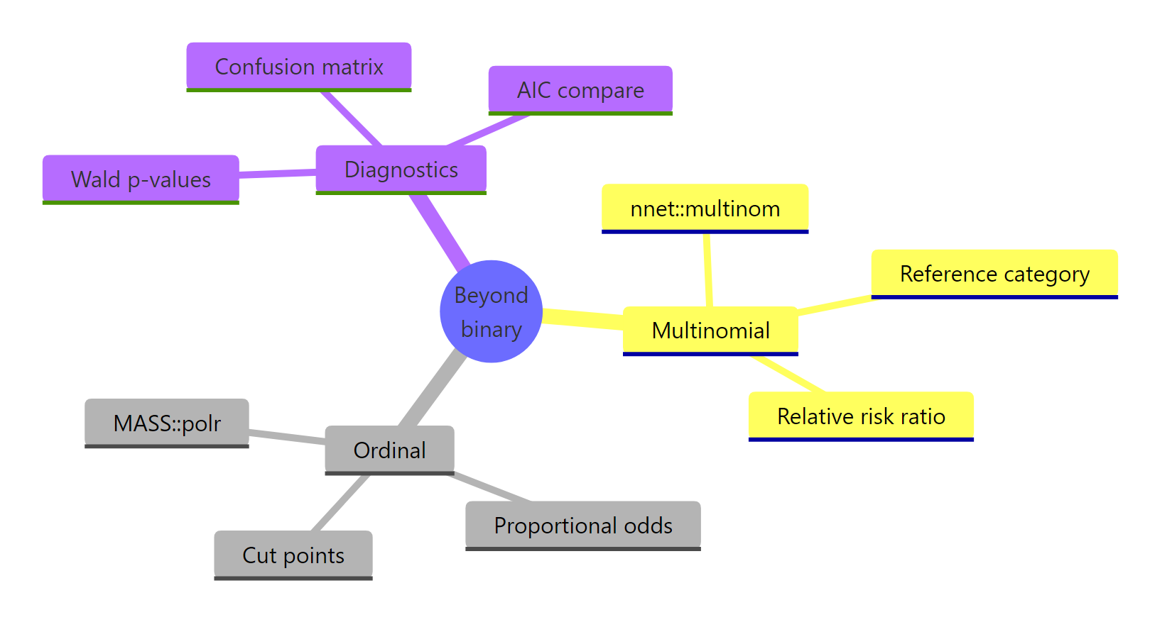
Figure 3: Models, key functions, and diagnostics covered in this tutorial.
| Outcome shape | Model | R function | Key diagnostic |
|---|---|---|---|
| 2 categories | Binary logistic | glm(family = binomial) |
Deviance, ROC, AUC |
| 3+ unordered | Multinomial logistic | nnet::multinom() |
Wald p-values, confusion matrix |
| 3+ ordered | Ordinal logistic | MASS::polr() |
Proportional odds (Brant, AIC vs multinom) |
Three takeaways:
- The number of categories and whether they are ranked decide the model. Misclassifying that choice costs accuracy or interpretability.
multinom()runs K-1 binary logits against a chosen reference class;polr()shares one slope across cut points to leverage the ranking.- Always validate ordinal fits against the proportional odds assumption before quoting odds ratios.
References
- UCLA OARC. Multinomial Logistic Regression | R Data Analysis Examples. Link
- UCLA OARC. Ordinal Logistic Regression | R Data Analysis Examples. Link
- Venables, W. N., and Ripley, B. D. Modern Applied Statistics with S, 4th Edition. Springer (2002). Chapter 7: Generalised Linear Models. Link
- Agresti, A. Categorical Data Analysis, 3rd Edition. Wiley (2013).
- nnet package documentation. multinom() reference. Link
- MASS package documentation. polr() reference. Link
- UVA Library. Visualizing the Effects of Proportional-Odds Logistic Regression. Link
Continue Learning
- Logistic Regression in R: the binary base case, with diagnostics, ROC, and AUC.
- Categorical Data in R: tables, mosaic plots, and chi-square tests for categorical predictors and outcomes.
- Odds Ratios and Relative Risk in R: companion piece for interpreting the exponentiated coefficients above.