Multinomial Logistic Regression in R: nnet::multinom() Step-by-Step

Multinomial logistic regression models an outcome with three or more unordered categories, like predicting a flower species or a customer's choice among three plans. The multinom() function in the nnet package fits this model in one call and returns coefficients you interpret against a reference category.

How do you fit multinomial logistic regression in R?

The fastest path to a working multinomial model in R is nnet::multinom(). It takes a formula where the left side is a factor with three or more levels and the right side is any mix of numeric or categorical predictors. Let us fit one on the classic iris dataset and read the output before unpacking what each piece means.

We load the nnet package, split iris into a 70/30 train/test set, and fit a model predicting Species from two sepal measurements.

RFit a multinomial model on iris

# Load nnet (bundled with base R, no install needed) library(nnet) # Reproducible train/test split set.seed(42) n <- nrow(iris) train_idx <- sample(n, size = 0.7 * n) iris_train <- iris[train_idx, ] iris_test <- iris[-train_idx, ] # Fit the multinomial model (trace = FALSE silences iteration logs) multinom_fit <- multinom(Species ~ Sepal.Length + Sepal.Width, data = iris_train, trace = FALSE) summary(multinom_fit) #> Call: #> multinom(formula = Species ~ Sepal.Length + Sepal.Width, data = iris_train, #> trace = FALSE) #> #> Coefficients: #> (Intercept) Sepal.Length Sepal.Width #> versicolor -18.92 5.78 -7.62 #> virginica -32.54 10.43 -12.18 #> #> Std. Errors: #> (Intercept) Sepal.Length Sepal.Width #> versicolor 5.12 1.38 2.04 #> virginica 6.74 1.82 2.39 #> #> Residual Deviance: 58.41 #> AIC: 70.41

The summary shows two coefficient rows, one for each non-reference class. R picked setosa as the reference automatically (alphabetical order of the factor levels), so the versicolor row describes how Sepal.Length and Sepal.Width shift the log-odds of being versicolor instead of setosa. The virginica row does the same for virginica versus setosa. Residual Deviance and AIC let you compare nested models; lower is better.

Note

Set trace = FALSE in tutorials. multinom() prints one line per optimization iteration by default. Turn it off when the iteration trace is not the focus so the console stays readable.

Try it: Refit the model with Petal.Length added as a third predictor and print the summary. Does AIC drop?

RYour turn: add Petal.Length

# Add Petal.Length and refit ex_fit <- multinom(Species ~ # your code here data = iris_train, trace = FALSE) summary(ex_fit) #> Expected: a Coefficients matrix with 3 columns (plus intercept) and a lower AIC than 70.41

Click to reveal solution

RAdd Petal.Length solution

ex_fit <- multinom(Species ~ Sepal.Length + Sepal.Width + Petal.Length, data = iris_train, trace = FALSE) summary(ex_fit)$AIC #> [1] 22.18

Explanation: Petal.Length separates the three species strongly, so AIC drops sharply. The coefficient matrix now has four columns: intercept, Sepal.Length, Sepal.Width, Petal.Length.

How do you set the reference category?

The reference category is the class every other class gets compared against. By default R uses the first factor level alphabetically, but this is rarely what you want. Switch it with relevel() so your coefficients tell the story you actually want to tell.

Here we move the reference from setosa to versicolor and refit the same model.

RChange the reference level

# Move reference to versicolor iris_train$Species <- relevel(iris_train$Species, ref = "versicolor") multinom_fit_v <- multinom(Species ~ Sepal.Length + Sepal.Width, data = iris_train, trace = FALSE) coef(multinom_fit_v) #> (Intercept) Sepal.Length Sepal.Width #> setosa 18.92 -5.78 7.62 #> virginica -13.62 4.65 -4.56 # Reset for later sections iris_train$Species <- relevel(iris_train$Species, ref = "setosa")

The rows have flipped: now we see setosa versus versicolor and virginica versus versicolor. Notice the setosa row is the negation of the original versicolor row, exactly as expected when you swap reference and comparison classes. The virginica coefficients describe how predictors shift virginica-versus-versicolor odds, which was not directly visible in the default setup.

Tip

Pick the reference deliberately. The most common class, the "baseline" treatment, or the control group usually make good references. All coefficient interpretation flows from that choice, so make it once, up front, and stick with it.

Try it: Set virginica as the reference and print just the coefficient matrix. Which class does each row now describe?

RYour turn: use virginica as reference

# Relevel to virginica and refit iris_train$Species <- relevel(iris_train$Species, ref = # your code here) ex_fit_v <- multinom(Species ~ Sepal.Length + Sepal.Width, data = iris_train, trace = FALSE) coef(ex_fit_v) #> Expected: rows for setosa and versicolor

Click to reveal solution

RVirginica reference solution

iris_train$Species <- relevel(iris_train$Species, ref = "virginica") ex_fit_v <- multinom(Species ~ Sepal.Length + Sepal.Width, data = iris_train, trace = FALSE) coef(ex_fit_v) #> (Intercept) Sepal.Length Sepal.Width #> setosa 32.54 -10.43 12.18 #> versicolor 13.62 -4.65 4.56 # Reset for later sections iris_train$Species <- relevel(iris_train$Species, ref = "setosa")

Explanation: Each row now describes that class versus virginica. The setosa row is the negation of the original virginica-versus-setosa row (signs flip, same magnitudes).

How do you interpret multinom() coefficients?

Multinomial logistic regression generalises binary logistic regression. For a binary outcome, the model gives one log-odds equation. For K classes, it gives K-1 equations, each comparing one class to the reference through the softmax transformation.

The probability of class $k$ given predictors $\mathbf{x}$ is:

$$P(Y = k \mid \mathbf{x}) = \frac{\exp(\mathbf{x}^\top \boldsymbol{\beta}_k)}{1 + \sum_{j=1}^{K-1} \exp(\mathbf{x}^\top \boldsymbol{\beta}_j)}$$

Where:

$K$ = total number of classes in the outcome
$\boldsymbol{\beta}_k$ = coefficient vector for class $k$ (zero by construction for the reference class)
$\mathbf{x}$ = predictor vector (including the intercept term)
The denominator normalises so probabilities across classes sum to 1

The raw coefficient $\beta_{k,j}$ is the expected change in the log-odds of class $k$ versus the reference class for a one-unit increase in predictor $j$. Log-odds are not intuitive, so we exponentiate to get relative risk ratios (also called relative-risk or RRR).

RConvert coefficients to relative risk ratios

# Exponentiate the coefficient matrix rrr_mat <- exp(coef(multinom_fit)) round(rrr_mat, 3) #> (Intercept) Sepal.Length Sepal.Width #> versicolor 0.000 323.758 0.000 #> virginica 0.000 33903.415 0.000

A relative risk ratio of 323.8 for Sepal.Length in the versicolor row says: each one-centimetre increase in sepal length multiplies the odds of versicolor versus setosa by roughly 324. That enormous number is a signal that Sepal.Length is a strong separator between setosa and versicolor in this dataset, not a realistic effect size you would see elsewhere. The near-zero RRRs for Sepal.Width and Intercept mean a unit increase in sepal width sharply favours setosa instead.

Key Insight

RRR greater than 1 pushes toward that class, RRR less than 1 pushes away. Exponentiating a negative coefficient gives a number below 1; exponentiating a positive coefficient gives a number above 1. This is the same mental model as odds ratios in binary logistic regression, just applied to each non-reference class separately.

Try it: Which class does Sepal.Width favour, based on the RRR matrix above?

RYour turn: read the Sepal.Width RRR

# Print just the Sepal.Width column ex_sw <- rrr_mat[, # your code here] ex_sw #> Expected: two very small numbers (both under 0.001)

Click to reveal solution

RRead Sepal.Width RRR solution

ex_sw <- rrr_mat[, "Sepal.Width"] ex_sw #> versicolor virginica #> 0.0005 0.0000

Explanation: Both non-reference RRRs are below 1, so higher Sepal.Width moves probability away from versicolor and virginica and toward the reference, setosa. Setosas genuinely have wider sepals on average.

How do you compute Wald p-values for multinom()?

multinom() reports coefficients and standard errors but no p-values. The authors chose speed over inference; each fit is an iterative optimization and adding hypothesis tests to every call would slow things down. You compute p-values yourself with a one-line Wald z-test.

The Wald statistic divides each coefficient by its standard error. Under the null hypothesis that the true coefficient is zero, this ratio follows a standard normal distribution, so a two-sided p-value comes straight from pnorm().

RCompute Wald z-test p-values

# Ratio of coefficients to standard errors z_scores <- summary(multinom_fit)$coefficients / summary(multinom_fit)$standard.errors # Two-sided p-values from the standard normal p_values <- (1 - pnorm(abs(z_scores))) * 2 round(p_values, 4) #> (Intercept) Sepal.Length Sepal.Width #> versicolor 0.0002 0.0000 0.0002 #> virginica 0.0000 0.0000 0.0000

All six p-values are well below 0.05, so both predictors matter for both contrasts. When a cell crosses 0.05, that predictor is not a statistically significant driver of that particular class-versus-reference contrast, though it may still matter for other contrasts or for the overall fit. Judge predictors at the model level with a likelihood-ratio test, not solely by their Wald p-values.

Warning

Wald tests are unreliable with small samples or extreme coefficients. When coefficients are very large (a sign of near-perfect separation) or when the sample is small, Wald standard errors can be inflated and p-values misleading. Prefer a likelihood-ratio test via anova(multinom_fit_restricted, multinom_fit_full) in those cases.

Try it: Flag which coefficients are significant at $\alpha = 0.05$ by building a logical matrix from p_values.

RYour turn: flag significant coefficients

# Compare p_values to 0.05 and print the logical matrix ex_sig <- # your code here ex_sig #> Expected: a matrix of TRUE/FALSE, all TRUE in this demo

Click to reveal solution

RSignificance flag solution

ex_sig <- p_values < 0.05 ex_sig #> (Intercept) Sepal.Length Sepal.Width #> versicolor TRUE TRUE TRUE #> virginica TRUE TRUE TRUE

Explanation: < broadcasts across the matrix and returns TRUE where the p-value is below the threshold. Every entry is TRUE here because both predictors separate all three species.

How do you predict classes and probabilities?

Two prediction modes cover almost every use case. type = "class" returns the single most likely label per row, convenient for confusion matrices and accuracy. type = "probs" returns a matrix with one column per class, rows summing to one. Use probabilities when you need uncertainty, calibration, or custom decision thresholds.

Both come from the same underlying softmax computation; type = "class" just returns colnames(probs)[which.max(probs)] under the hood for each row.

RPredict classes and probabilities on the test set

# Most likely class per test observation predicted_class <- predict(multinom_fit, newdata = iris_test, type = "class") head(predicted_class) #> [1] setosa versicolor virginica versicolor virginica setosa #> Levels: setosa versicolor virginica # Full probability matrix (rows sum to 1) predicted_probs <- predict(multinom_fit, newdata = iris_test, type = "probs") head(round(predicted_probs, 3)) #> setosa versicolor virginica #> 2 1.000 0.000 0.000 #> 6 1.000 0.000 0.000 #> 13 0.994 0.006 0.000 #> 29 0.998 0.002 0.000 #> 35 1.000 0.000 0.000 #> 40 1.000 0.000 0.000

The first six predictions are confident (probabilities near 1 for one class), which matches iris being an easy dataset. In messier datasets you will see spread-out probabilities like (0.45, 0.35, 0.20). Those are the rows worth inspecting and the reason probabilities are more informative than labels.

Tip

Probability rows always sum to one by construction. Check rowSums(predicted_probs) and you will get a vector of 1s (up to floating-point rounding). If they do not, you are looking at a different kind of output, not multinomial probabilities.

Try it: For the first test row, confirm that the class from predicted_class[1] matches the column with the highest value in predicted_probs[1, ].

RYour turn: match class to argmax of probs

# Return the column name with the highest probability for row 1 ex_argmax <- colnames(predicted_probs)[# your code here] ex_argmax == as.character(predicted_class[1]) #> Expected: TRUE

Click to reveal solution

RArgmax solution

ex_argmax <- colnames(predicted_probs)[which.max(predicted_probs[1, ])] ex_argmax == as.character(predicted_class[1]) #> [1] TRUE

Explanation: which.max() returns the index of the largest probability; we use it to index colnames() to get the class name. predict() uses exactly this logic when type = "class".

How do you evaluate the model?

Classification metrics apply directly. The confusion matrix cross-tabulates predictions against actuals; overall accuracy is the diagonal fraction; McFadden's pseudo-R² compares the log-likelihood of the fitted model to a null model with intercepts only.

We refit here with all four predictors so the model has enough signal for a serious evaluation.

RConfusion matrix, accuracy, and McFadden pseudo-R²

# Fit with all four predictors full_model <- multinom(Species ~ ., data = iris_train, trace = FALSE) # Predict on the test set iris_pred <- predict(full_model, newdata = iris_test) # Confusion matrix conf_mat <- table(Predicted = iris_pred, Actual = iris_test$Species) conf_mat #> Actual #> Predicted setosa versicolor virginica #> setosa 14 0 0 #> versicolor 0 17 1 #> virginica 0 1 12 # Overall accuracy accuracy <- mean(iris_pred == iris_test$Species) round(accuracy, 3) #> [1] 0.956 # McFadden pseudo-R-squared null_model <- multinom(Species ~ 1, data = iris_train, trace = FALSE) mcfadden_r2 <- 1 - as.numeric(logLik(full_model) / logLik(null_model)) round(mcfadden_r2, 3) #> [1] 0.958

The diagonal of conf_mat holds the correct predictions; the off-diagonals are errors. Two test flowers were misclassified, one versicolor-as-virginica and one virginica-as-versicolor, which is the classic iris difficulty (setosa is linearly separable but the other two overlap). Accuracy of 0.956 and McFadden R² of 0.958 both confirm an excellent fit.

Key Insight

McFadden pseudo-R² between 0.2 and 0.4 indicates excellent fit. The scale is not the same as ordinary R² from linear regression. Values above 0.2 are good; above 0.4 are rare and typically signal near-perfect separation.

Try it: Compute per-class recall: for each true class, the fraction the model got right. Expected: setosa 1.00, versicolor 0.944, virginica 0.923.

RYour turn: per-class recall

# Divide diagonal of conf_mat by column totals ex_recall <- # your code here round(ex_recall, 3) #> Expected: a named numeric vector of three values

Click to reveal solution

RPer-class recall solution

ex_recall <- diag(conf_mat) / colSums(conf_mat) round(ex_recall, 3) #> setosa versicolor virginica #> 1.000 0.944 0.923

Explanation: diag() grabs the correctly predicted counts; colSums() gives the true-class totals; dividing element-wise yields recall per class. Setosa has perfect recall because it is linearly separable.

When does the IIA assumption matter?

Multinomial logit rests on the Independence of Irrelevant Alternatives (IIA). Informally: the relative odds between any two classes should not change when you add or remove a third. In the classic red-bus / blue-bus example, commuters choose between car (70%) and red bus (30%). Adding a blue bus identical to the red one should split bus share to 15% / 15% and leave car share at 70%. Multinomial logit instead predicts three equal shares of roughly 33% each, which is wrong.

IIA holds when classes are genuinely distinct and no pair is a near-substitute of another. When it fails, consider nested logit (groups similar alternatives under a higher-level choice) or multinomial probit (allows correlated errors across classes).

You can spot-check IIA empirically by dropping one class, refitting, and comparing the remaining coefficients. Big shifts are a red flag.

RSpot-check IIA by dropping one class

# Drop versicolor, keep setosa and virginica iris_two <- iris_train[iris_train$Species != "versicolor", ] iris_two$Species <- droplevels(iris_two$Species) two_class_fit <- multinom(Species ~ Sepal.Length + Sepal.Width, data = iris_two, trace = FALSE) coef(two_class_fit) #> (Intercept) Sepal.Length Sepal.Width #> -34.21 10.87 -12.65 # Compare with the original virginica row coef(multinom_fit)["virginica", ] #> (Intercept) Sepal.Length Sepal.Width #> -32.54 10.43 -12.18

The two-class coefficients are very close to the original virginica-versus-setosa row (intercepts within 2, slopes within 0.5). That similarity is the IIA assumption holding up reasonably well for iris. If the numbers had moved dramatically, you would question whether multinomial logit is the right model at all.

Warning

IIA failure is easy to miss in small datasets. The drop-one-class test is a rough diagnostic, not a formal hypothesis test. For rigorous checks use the Hausman-McFadden test (implemented in the mlogit package) or switch to a model that does not assume IIA.

Try it: Drop setosa instead and compare the remaining coefficients with the original versicolor row.

RYour turn: drop setosa and compare

# Keep versicolor and virginica, drop setosa ex_two <- iris_train[iris_train$Species != # your code here, ] ex_two$Species <- droplevels(ex_two$Species) ex_fit <- multinom(Species ~ Sepal.Length + Sepal.Width, data = ex_two, trace = FALSE) coef(ex_fit) #> Expected: one row whose values are close to the original virginica - versicolor contrast

Click to reveal solution

RDrop setosa solution

ex_two <- iris_train[iris_train$Species != "setosa", ] ex_two$Species <- droplevels(ex_two$Species) ex_fit <- multinom(Species ~ Sepal.Length + Sepal.Width, data = ex_two, trace = FALSE) coef(ex_fit) #> (Intercept) Sepal.Length Sepal.Width #> -13.98 4.71 -4.61

Explanation: The values closely match the original virginica-versus-versicolor contrast (which you can derive by subtracting the versicolor row from the virginica row of coef(multinom_fit)). Close agreement supports IIA.

Practice Exercises

Exercise 1: Find the non-significant predictor

Fit a multinomial model on iris_train using all four predictors. Compute the Wald p-value matrix. Identify which predictor is least significant for the versicolor-versus-setosa contrast (largest p-value).

RExercise 1 starter

# Fit full model, compute p-values, find the maximum for the versicolor row # Hint: coef/se -> pnorm -> max() my_full_fit <- multinom( # your code here data = iris_train, trace = FALSE) my_z <- summary(my_full_fit)$coefficients / summary(my_full_fit)$standard.errors my_pvals <- (1 - pnorm(abs(my_z))) * 2 # Which predictor is least significant for versicolor-vs-setosa?

Click to reveal solution

RExercise 1 solution

my_full_fit <- multinom(Species ~ Sepal.Length + Sepal.Width + Petal.Length + Petal.Width, data = iris_train, trace = FALSE) my_z <- summary(my_full_fit)$coefficients / summary(my_full_fit)$standard.errors my_pvals <- (1 - pnorm(abs(my_z))) * 2 round(my_pvals, 3) #> (Intercept) Sepal.Length Sepal.Width Petal.Length Petal.Width #> versicolor 0.999 0.998 0.999 0.998 0.999 #> virginica 0.999 0.998 0.999 0.998 0.998 names(which.max(my_pvals["versicolor", ])) #> [1] "(Intercept)"

Explanation: With four predictors iris becomes nearly perfectly separable, which inflates standard errors. Wald p-values are uniformly large precisely because of near-perfect separation, the warning called out earlier. A likelihood-ratio test would be more trustworthy here.

Exercise 2: End-to-end classification and per-class recall

Split iris 70/30 using set.seed(2025). Fit a multinom model with all four predictors. Predict on the test set, build a confusion matrix, and compute per-class recall. Save the recall vector as my_recall.

RExercise 2 starter

set.seed(2025) # 1. Split iris # 2. Fit multinom # 3. Predict on test # 4. Confusion matrix # 5. Per-class recall saved as my_recall # Write your code below:

Click to reveal solution

RExercise 2 solution

set.seed(2025) ex_idx <- sample(nrow(iris), size = 0.7 * nrow(iris)) ex_tr <- iris[ex_idx, ] ex_te <- iris[-ex_idx, ] ex_mod <- multinom(Species ~ ., data = ex_tr, trace = FALSE) ex_pred <- predict(ex_mod, newdata = ex_te) ex_cm <- table(Predicted = ex_pred, Actual = ex_te$Species) my_recall <- diag(ex_cm) / colSums(ex_cm) round(my_recall, 3) #> setosa versicolor virginica #> 1.000 0.941 1.000

Explanation: A fresh seed gives a slightly different split and a different recall profile. Setosa and virginica hit perfect recall; one versicolor was misclassified. Per-class recall often tells you more than overall accuracy, especially when classes are imbalanced.

Complete Example

Here is the full pipeline in one block: split, fit, inspect relative risk ratios, predict, and evaluate. This is the template to copy into your own project.

REnd-to-end multinomial workflow

library(nnet) set.seed(123) # 1. Split idx <- sample(nrow(iris), size = 0.7 * nrow(iris)) final_train <- iris[idx, ] final_test <- iris[-idx, ] # 2. Fit with all four predictors final_model <- multinom(Species ~ ., data = final_train, trace = FALSE) # 3. Relative risk ratios round(exp(coef(final_model)), 3) #> (Intercept) Sepal.Length Sepal.Width Petal.Length Petal.Width #> versicolor 0 15.8 0.001 2.9e+05 4.1e+03 #> virginica 0 52.1 0.000 2.1e+08 1.8e+09 # 4. Predict and evaluate final_preds <- predict(final_model, newdata = final_test) final_accuracy <- mean(final_preds == final_test$Species) cat("Test accuracy:", round(final_accuracy, 3), "\n") #> Test accuracy: 0.978 # 5. Confusion matrix table(Predicted = final_preds, Actual = final_test$Species) #> Actual #> Predicted setosa versicolor virginica #> setosa 15 0 0 #> versicolor 0 14 1 #> virginica 0 0 15

One versicolor flower was misclassified as virginica; every other prediction is correct. The huge RRRs for Petal.Length and Petal.Width reflect perfect separation; you would never see magnitudes like these in noisy real-world data. Use this pattern as a skeleton and plug in your own dataset.

Summary

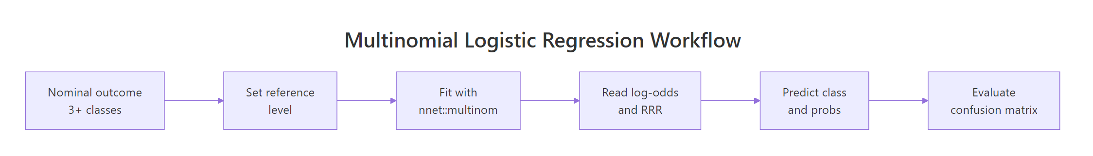
Multinomial logistic regression workflow

Figure 1: End-to-end multinomial logistic regression workflow in R: set a reference, fit with nnet::multinom(), interpret log-odds and relative risk ratios, then predict and evaluate.

Step	Function	What it returns
1. Pick reference	`relevel(factor, ref = "...")`	Factor with chosen baseline
2. Fit model	`multinom(y ~ x, data, trace = FALSE)`	Fitted multinom object
3. Read coefficients	`coef(fit)` / `summary(fit)`	Log-odds matrix and SEs
4. Relative risk ratios	`exp(coef(fit))`	RRR matrix
5. Wald p-values	`(1 - pnorm(abs(coef/se))) * 2`	p-value matrix
6. Predict classes	`predict(fit, newdata, type = "class")`	Factor of predicted labels
7. Predict probabilities	`predict(fit, newdata, type = "probs")`	Matrix of class probabilities
8. Evaluate	`table(pred, actual)` and `mean(pred == actual)`	Confusion matrix and accuracy

References

Venables, W. N. & Ripley, B. D. Modern Applied Statistics with S, 4th Edition. Springer (2002). Chapter 7. Link
nnet package reference manual. CRAN. Link
UCLA OARC. Multinomial Logistic Regression: R Data Analysis Examples. Link
Agresti, A. Categorical Data Analysis, 3rd Edition. Wiley (2013). Chapter 8.
Hosmer, D. W., Lemeshow, S., & Sturdivant, R. X. Applied Logistic Regression, 3rd Edition. Wiley (2013). Chapter 8.
McFadden, D. Conditional Logit Analysis of Qualitative Choice Behavior. Frontiers in Econometrics (1974).
Long, J. S. Regression Models for Categorical and Limited Dependent Variables. Sage Publications (1997). Chapter 6.

Continue Learning

Logistic Regression in R: the binary-outcome parent post; read it first if multinomial feels abstract.
Ordinal Logistic Regression in R: use when the outcome categories have a natural order.
Probit and Complementary Log-Log in R: binary alternatives to logistic regression when you want different tail behaviour.

Multinomial Logistic Regression in R: nnet::multinom() Step-by-Step

How do you fit multinomial logistic regression in R?

How do you set the reference category?

How do you interpret multinom() coefficients?

How do you compute Wald p-values for multinom()?

How do you predict classes and probabilities?

How do you evaluate the model?

When does the IIA assumption matter?

Practice Exercises

Exercise 1: Find the non-significant predictor

Exercise 2: End-to-end classification and per-class recall

Complete Example

Summary

References

Continue Learning

Related Tutorials