Spatial Data in R with sf: Shapefiles, CRS Transformation, and ggplot2 Maps

The sf (simple features) package is R's modern standard for working with spatial data, points, lines, and polygons stored as tidy data frames. It replaces the older sp package and connects seamlessly with dplyr for data manipulation and ggplot2 for mapping.

What does spatial data look like in R?

Spatial data connects locations on Earth to attributes you care about, city populations, river lengths, country boundaries. In R, the sf package stores this data as a regular data frame with one special column: a geometry column that holds the coordinates.

Let's create a simple spatial dataset and see what that looks like.

Notice how it looks just like a regular data frame, except for that geometry column on the right. Each row stores a POINT with longitude and latitude. The header tells you the CRS (WGS 84, which is standard GPS coordinates) and the bounding box (the rectangle that contains all your points).

The built-in plot() function gives you a quick look at the data. It creates one panel per attribute column.

The plot shows three mini-maps (one for each attribute column). Each point is colored by the attribute value. This is useful for a quick sanity check, but for publication-quality maps you'll want ggplot2, we'll get there in a later section.

What are the sf geometry types?

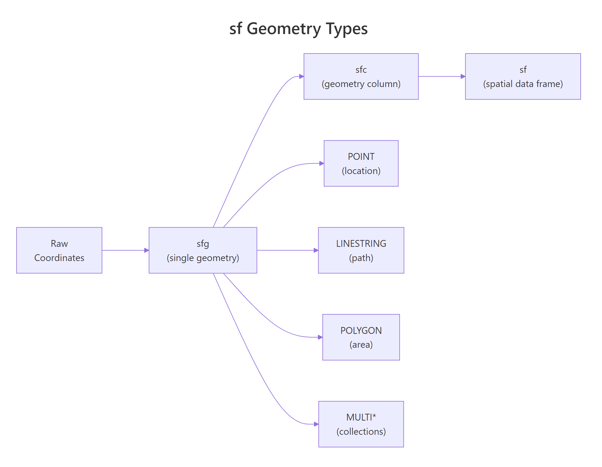
sf supports several geometry types. The three you'll use most often are POINT (a single location), LINESTRING (a connected path), and POLYGON (a closed boundary). Each maps to a real-world feature.

Let's create a LINESTRING to represent a simplified river path.

The river is stored as a sequence of coordinate pairs connected in order. Now let's make a POLYGON, a closed shape where the first and last coordinates must match.

Now let's plot all three geometry types together to see how they layer.

The polygon (lake) renders as a filled shape, the linestring (river) as a line, and the point (Chicago) as a dot. ggplot2's geom_sf() figures out the correct visual representation automatically based on the geometry type.

Figure 1: The four core geometry types in sf and how they nest: sfg → sfc → sf.

How do you read spatial data files into R?

In your own projects, you'll usually start by reading spatial files from disk. The sf package's st_read() function handles all major formats, shapefiles, GeoJSON, GeoPackage, KML, and more.

Here's the pattern for the most common formats:

A practical workaround for getting real map data without files is to convert R's built-in map data to sf. The maps package contains world, US state, and country boundaries.

Now world_sf is a proper sf object with MULTIPOLYGON geometries for each country. You can use it exactly like data loaded from a shapefile, filter countries, transform projections, or plot with ggplot2.

What is a coordinate reference system and why does it matter?

Every spatial dataset needs a coordinate reference system (CRS), the set of rules that tells R how the numbers in your geometry column relate to actual locations on Earth. Without a CRS, your coordinates are just abstract numbers.

There are two families of CRS to know:

Geographic CRS stores positions as longitude and latitude on the globe's curved surface. Projected CRS flattens the globe onto a 2D plane, like peeling an orange and pressing the skin flat. Each projection distorts something (area, shape, distance, or direction), so you pick the one that preserves what you care about.

Let's check the CRS on our world map.

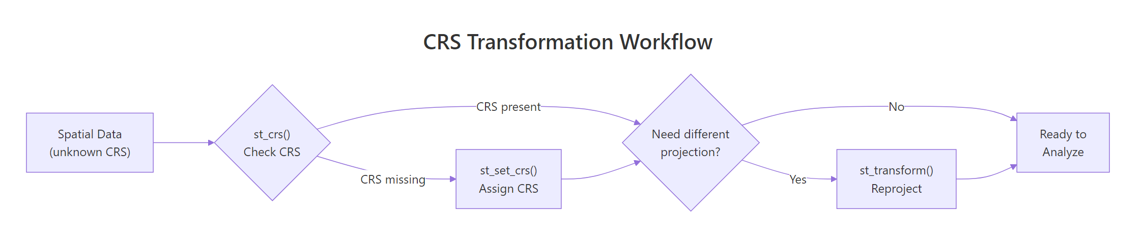
The output confirms this is WGS 84 (EPSG:4326), the most common geographic CRS. If you create spatial data from coordinates and forget to set a CRS, you'll get NA. Let's see how to assign one.

Figure 2: Decision flow for checking, assigning, and transforming a CRS.

How do you transform between coordinate systems?

st_set_crs() assigns a CRS to data that doesn't have one (it labels the coordinates). st_transform() reprojects the data, it recalculates every coordinate into a different coordinate system. This is the function you'll use to switch between projections.

A common scenario: your data is in WGS 84 (degrees), but you need meters for distance or area calculations. Let's transform the US states from WGS 84 to Albers Equal Area, a projection designed for the contiguous US that preserves area proportions.

The WGS 84 coordinates are in degrees (longitude, latitude). After transformation to Albers, they're in meters, much better for computing areas and distances.

Let's see the visual difference between the two projections.

In the WGS 84 version, the map looks stretched east-west. The Albers projection gives the familiar, proportionally correct US shape.

How do you create maps with geom_sf() in ggplot2?

geom_sf() is the ggplot2 layer built for sf objects. It automatically picks the right visual, polygons get filled, lines get stroked, points get plotted as dots. You use it exactly like any other ggplot layer, with aesthetic mappings for fill, color, size, and more.

Let's create a basic map of US states and then build up from there.

theme_void() strips away axes and gridlines, perfect for maps where coordinate labels add clutter. Now let's layer two sf objects: states as polygons and cities as points on top.

Each geom_sf() layer can come from a different sf object. ggplot2 handles CRS alignment automatically, if the layers have different projections, it reprojects to match the first one.

Now let's build a choropleth map, states colored by a data variable.

scale_fill_viridis_c() provides colorblind-friendly palettes that work well for maps. The option argument lets you pick from "viridis", "magma", "plasma", "inferno", and "cividis".

How do you use dplyr verbs with sf objects?

One of sf's biggest advantages over older spatial packages is that it works natively with dplyr. You can filter(), mutate(), group_by(), and summarise() exactly like you would with a regular data frame, the geometry column comes along for the ride.

Let's filter and transform our US states data.

The geometry column survived the filter, no extra steps needed. Now here's the powerful part: summarise() on sf objects dissolves (merges) geometries by group. Individual state boundaries disappear and you get one polygon per group.

The 49 individual state polygons merged into 4 region polygons. This is called "dissolving" in GIS terminology, sf does it automatically when you summarise by group.

Practice Exercises

Exercise 1: City population map

Create an sf object of 5 world cities with columns for name, country, and population (in millions). Set the CRS to WGS 84. Then plot them on top of the world map using geom_sf(), sizing points by population and coloring them by country.

Exercise 2: State area choropleth

Using the us_albers sf object (already projected), compute each state's area with st_area() and create a choropleth map colored by area. Add a title, use scale_fill_viridis_c(), and apply theme_void().

Exercise 3: European map with labels

Transform world_sf to Robinson projection ("+proj=robin"). Filter to keep only European countries (use approximate bounding box: longitude -25 to 45, latitude 35 to 72). Create a styled map with geom_sf_text() for country labels.

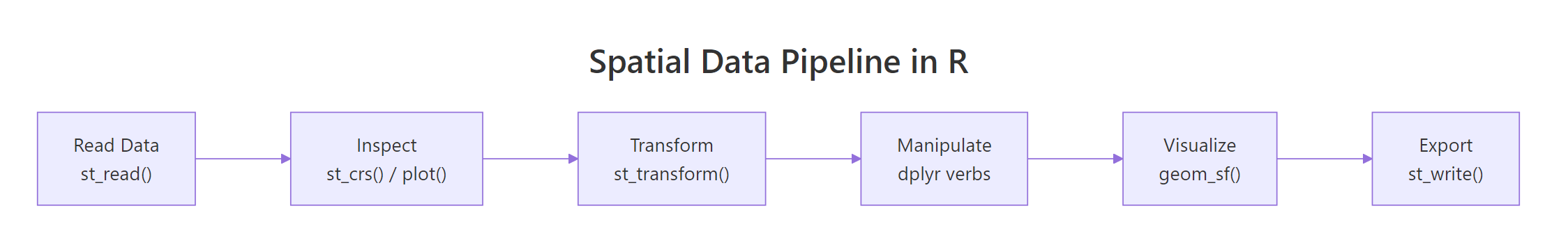
Putting It All Together

Let's walk through a complete spatial analysis workflow, from raw data to a polished, publication-ready map.

The goal: create a choropleth map of US states colored by area, with major cities overlaid as sized points, all in a proper equal-area projection.

This workflow covers every core concept from the tutorial: creating sf objects, checking and transforming CRS, computing spatial measurements, layering multiple geometries, and styling with ggplot2.

Summary

Here's a quick reference for the sf functions covered in this tutorial:

Key takeaways:

• sf objects are data frames with a geometry column, use them with any dplyr verb
• Always check your CRS with st_crs() before analysis or plotting
• Use st_set_crs() to label coordinates; use st_transform() to reproject them
• geographic CRS (WGS 84) stores degrees; projected CRS stores meters, pick projected for area/distance calculations
• geom_sf() in ggplot2 automatically handles geometry rendering and CRS alignment
• summarise() on sf objects dissolves (merges) geometries by group
• The maps package provides built-in boundary data you can convert with st_as_sf()

Figure 3: A typical spatial data pipeline from reading to visualization.

References

1. Pebesma, E., sf: Simple Features for R. CRAN. Link
2. Pebesma, E. & Bivand, R., Spatial Data Science. Chapter 7: Introduction to sf. Link
3. Wickham, H., ggplot2: geom_sf() reference. Link
4. EPSG.io, Coordinate Reference System database. Link
5. Lovelace, R., Nowosad, J., Muenchow, J., Geocomputation with R. Chapter 2: Geographic data in R. Link
6. r-spatial.org, Drawing beautiful maps programmatically with R, sf and ggplot2. Link
7. sf CRAN package documentation, Version 1.1-0. Link

Continue Learning

• ggplot2 Getting Started, Master the grammar of graphics that geom_sf() builds upon.
• ggplot2 Colours, Customize color palettes for choropleth maps and themed visualizations.
• ggplot2 Themes, Style your maps with custom themes for publication-quality output.