Sample Size in R: Calculate Your N Before You Collect a Single Observation

Sample size planning is calculating how many observations you need to reliably detect an effect of a given size, a decision made before collecting data, using the pwr package in R or simulation.

Introduction

Most studies don't fail because of bad analysis. They fail because of bad planning. A study with too few participants can't detect a real effect even when one exists, and you won't know until your results come back non-significant and it's too late to do anything about it. This is called an underpowered study, and it's one of the most common (and avoidable) problems in empirical research.

The good news is that the fix is simple: plan your sample size before you collect data. This process, called power analysis, takes the guesswork out of "how many participants do I need?" and replaces it with a principled calculation.

In this tutorial you'll learn how to use R's pwr package to calculate sample sizes for t-tests, proportions, ANOVA, and chi-squared tests. You'll also learn how to use simulation when pwr isn't flexible enough, and how to write the one-paragraph justification that grant reviewers and ethics boards actually want to see. All code runs interactively in your browser, no setup needed.

Note

The pwr package covers the most common test types. For mixed models, survival analysis, or complex repeated-measures designs, simulation (covered in Section 4) is your best tool. The pwrss package also extends coverage significantly.

What Is Statistical Power and Why Does It Matter Before You Collect Data?

Before any calculation, you need to understand the four quantities that are always involved in a power analysis. They're not independent, fix any three and the fourth is determined.

Effect size, how large the true difference is (e.g., Cohen's d for means, odds ratio for proportions)
Sample size (n), the number of observations per group
Alpha (α), the Type I error rate, usually 0.05 (your threshold for "statistically significant")
Power (1 − β), the probability of detecting the effect if it truly exists; the convention is 0.80

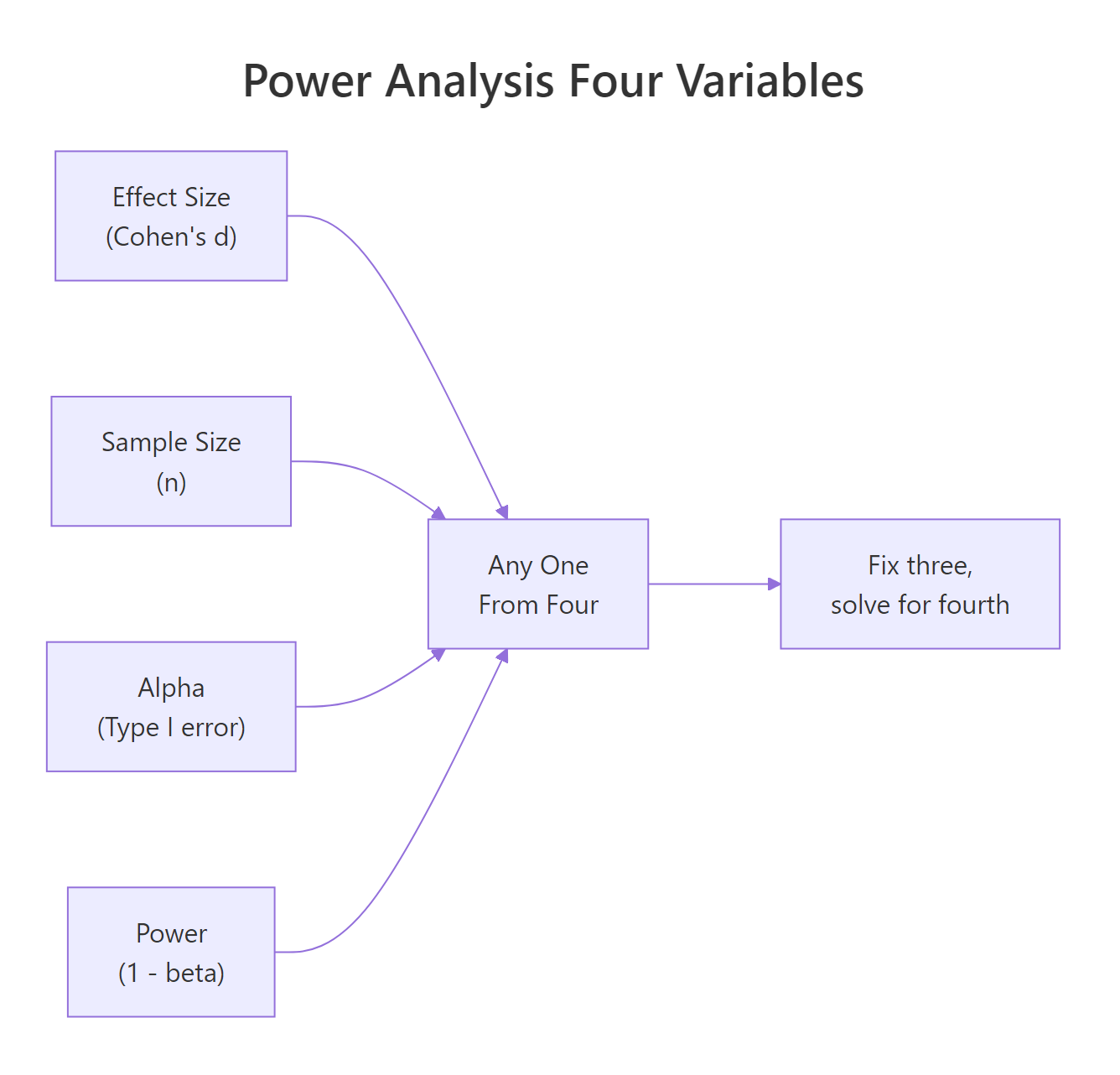
The four interdependent quantities in power analysis

Figure 1: The four interdependent quantities in power analysis. Fix any three and solve for the fourth.

Think of power as your study's sensitivity. A study with 80% power will detect a true effect 8 times out of 10. With 50% power, you're essentially flipping a coin. Most funding bodies and ethics boards expect at least 80% power; 90% is better for confirmatory trials.

Let's build intuition with a quick simulation. We'll generate data from two groups with a known difference, run a t-test, and count how often it's significant across 1,000 repetitions. That proportion is our empirical power.

RSimulate power for t-test

# Load pwr package and set seed for reproducibility library(pwr) set.seed(123) # Simulate power empirically: detect a medium effect (d = 0.5) with n = 50 per group n_per_group <- 50 d_true <- 0.5 n_sims <- 1000 p_values <- replicate(n_sims, { group1 <- rnorm(n_per_group, mean = 0, sd = 1) group2 <- rnorm(n_per_group, mean = d_true, sd = 1) t.test(group1, group2)$p.value }) empirical_power <- mean(p_values < 0.05) cat("Empirical power:", round(empirical_power, 3), "\n") #> Empirical power: 0.698

With n = 50 per group and a medium effect size (d = 0.5), we get about 70% power, below the 80% threshold. That means roughly 30% of studies with this design would fail to detect a real effect. This is why you calculate N before you start, not after.

Key Insight

Power is not about the data you have, it's about the data you plan to collect. Post-hoc power calculations (run after seeing non-significant results) are misleading and should never be reported. Plan prospectively.

Try it: Change n_per_group to 64 in the code above. What empirical power do you get? Is it closer to 80%?

RExercise: Power at n equals 64

# Try it: modify n_per_group and see how power changes ex_n <- 64 ex_p_values <- replicate(1000, { g1 <- rnorm(ex_n, mean = 0, sd = 1) g2 <- rnorm(ex_n, mean = 0.5, sd = 1) t.test(g1, g2)$p.value }) # your code here: compute mean(ex_p_values < 0.05) #> Expected: ~0.80

Click to reveal solution

RPower at 64 solution

ex_n <- 64 ex_p_values <- replicate(1000, { g1 <- rnorm(ex_n, mean = 0, sd = 1) g2 <- rnorm(ex_n, mean = 0.5, sd = 1) t.test(g1, g2)$p.value }) mean(ex_p_values < 0.05) #> [1] 0.801

Explanation: At n = 64 per group, a medium effect size (d = 0.5) yields approximately 80% power, right at the conventional threshold.

How Do You Calculate Sample Size for a t-Test in R?

The pwr package makes t-test sample size calculation a one-liner. The key function is pwr.t.test(). You provide three of the four quantities (effect size, n, alpha, power) and leave the fourth as NULL, that's the one R calculates.

The trickiest part is specifying the effect size. Cohen's d is the standardised mean difference: the expected difference between groups divided by the pooled standard deviation. Cohen proposed d = 0.2 as "small", 0.5 as "medium", and 0.8 as "large", but these are rough benchmarks. Always ground your effect size in prior literature or domain knowledge.

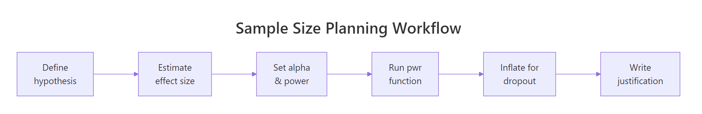
The six-step sample size planning workflow

Figure 2: The six-step sample size planning workflow, from hypothesis to written justification.

RTwo-sample t-test sample size

# Two-sample t-test: how many participants per group do we need? # Effect size d = 0.5 (medium), alpha = 0.05, power = 0.80 result_two_sample <- pwr.t.test( d = 0.5, sig.level = 0.05, power = 0.80, type = "two.sample" ) print(result_two_sample) #> #> Two-sample t test power calculation #> #> n = 63.77 #> d = 0.5 #> sig.level = 0.05 #> power = 0.8 #> alternative = two.sided #> #> NOTE: n is number in *each* group n_two_sample <- ceiling(result_two_sample$n) cat("You need", n_two_sample, "participants per group,", n_two_sample * 2, "total.\n") #> You need 64 participants per group, 128 total.

The output tells you n = 63.77, always round up to the next whole number. The note at the bottom is critical: n is per group, not total. A study with two groups needs 128 participants, not 64.

Now compare a one-sample test (measuring against a known baseline) with a paired design (measuring the same people twice). Paired designs are far more efficient because within-person variation is removed.

ROne-sample and paired designs

# One-sample t-test (comparing to a known value) n_one <- ceiling(pwr.t.test(d = 0.5, sig.level = 0.05, power = 0.80, type = "one.sample")$n) # Paired t-test (before/after in same participants) n_paired <- ceiling(pwr.t.test(d = 0.5, sig.level = 0.05, power = 0.80, type = "paired")$n) cat("One-sample:", n_one, "| Paired:", n_paired, "| Two-sample:", n_two_sample, "per group\n") #> One-sample: 34 | Paired: 34 | Two-sample: 64 per group

A paired design needs only 34 participants total for the same power. If your study design allows repeated measurements on the same individuals, paired testing can halve your recruitment burden.

It's also useful to see how power changes as n increases. A power curve makes this visual and is useful for grant applications.

RPower curve across sample sizes

# Power curve: power vs. sample size for d = 0.5 ns <- seq(10, 150, by = 5) powers <- sapply(ns, function(n) { pwr.t.test(n = n, d = 0.5, sig.level = 0.05, type = "two.sample")$power }) plot(ns, powers, type = "l", lwd = 2, col = "#4B6FA5", xlab = "Sample size per group", ylab = "Power", main = "Power curve: two-sample t-test (d = 0.5)") abline(h = 0.80, lty = 2, col = "red") abline(v = 64, lty = 2, col = "darkgreen") legend("bottomright", legend = c("Power", "80% threshold", "n = 64"), lty = c(1, 2, 2), col = c("#4B6FA5", "red", "darkgreen"))

The curve shows how power rises steeply at small n and flattens out. Beyond n = 100 per group, each additional participant buys very little extra power for this effect size.

Tip

Always inflate your calculated n for expected dropout. If you expect 15% attrition, divide the required n by (1 - 0.15): ceiling(64 / 0.85) gives 76 per group. Build this into your protocol from the start.

Try it: Calculate the sample size needed for a two-sample t-test with a small effect (d = 0.2) and 90% power. Save the result to ex_n_small.

RExercise: Small effect high power

# Try it: pwr.t.test for d=0.2, power=0.90, two.sample ex_n_small <- ceiling(pwr.t.test( d = 0.2, sig.level = 0.05, power = 0.90, type = "two.sample" # your code here )$n) cat("N per group:", ex_n_small) #> Expected: N per group: 527

Click to reveal solution

RSmall effect solution

ex_n_small <- ceiling(pwr.t.test( d = 0.2, sig.level = 0.05, power = 0.90, type = "two.sample" )$n) cat("N per group:", ex_n_small) #> [1] N per group: 527

Explanation: Small effects require very large samples. Detecting a d = 0.2 effect with 90% power needs over 500 participants per group, 1,054 total. This is why knowing your expected effect size before designing a study is so important.

How Do You Calculate Sample Size for Proportions, ANOVA, and Chi-Squared Tests?

Not every study compares means. pwr has dedicated functions for proportions (pwr.2p.test), ANOVA (pwr.anova.test), and chi-squared tests (pwr.chisq.test). Each uses a different effect size metric.

For proportions, Cohen's h is the effect size: ES.h(p1, p2) computes it from two proportions directly. For ANOVA, Cohen's f is used (f = 0.10 small, 0.25 medium, 0.40 large). For chi-squared, Cohen's w (w = 0.10 small, 0.30 medium, 0.50 large).

RSample size for two proportions

# --- Proportions: comparing two rates (e.g., 30% vs 45% conversion) --- h <- ES.h(p1 = 0.30, p2 = 0.45) # Cohen's h n_prop <- ceiling(pwr.2p.test(h = h, sig.level = 0.05, power = 0.80)$n) cat("Proportions, Cohen's h:", round(h, 3), "| N per group:", n_prop, "\n") #> Proportions, Cohen's h: 0.314 | N per group: 81

RANOVA and chi-squared sample size

# --- One-way ANOVA: 3 groups, medium effect (f = 0.25) --- n_anova <- ceiling(pwr.anova.test(k = 3, f = 0.25, sig.level = 0.05, power = 0.80)$n) cat("ANOVA (3 groups), N per group:", n_anova, "| Total:", n_anova * 3, "\n") #> ANOVA (3 groups), N per group: 53 | Total: 159 # --- Chi-squared: small effect (w = 0.10), 4 categories --- n_chisq <- ceiling(pwr.chisq.test(w = 0.10, df = 3, sig.level = 0.05, power = 0.80)$N) cat("Chi-squared (df=3), Total N:", n_chisq, "\n") #> Chi-squared (df=3), Total N: 1194

The chi-squared result (N = 1194) is a reminder that detecting small associations in contingency tables requires very large samples. If your study is testing a small frequency difference, plan accordingly.

Key Insight

Effect size conventions (small/medium/large) were meant as fallbacks, not defaults. Cohen himself called them "a convention adopted only when no better basis for estimating the ES index is available." Always prefer an effect size derived from a pilot study, prior literature, or the smallest clinically meaningful difference.

Try it: A clinical study expects 40% of patients to respond to treatment A and 55% to treatment B. Calculate the sample size per group needed at 80% power.

RExercise: Proportions 40 vs 55

# Try it: use ES.h() and pwr.2p.test() ex_h <- ES.h(p1 = 0.40, p2 = 0.55) ex_n_prop <- ceiling(pwr.2p.test( h = ex_h, sig.level = 0.05, power = 0.80 # your code here )$n) cat("N per group:", ex_n_prop) #> Expected: N per group: 97

Click to reveal solution

RProportions sample size solution

ex_h <- ES.h(p1 = 0.40, p2 = 0.55) ex_n_prop <- ceiling(pwr.2p.test(h = ex_h, sig.level = 0.05, power = 0.80)$n) cat("N per group:", ex_n_prop) #> [1] N per group: 97

Explanation: ES.h() computes Cohen's h from the two proportions (h ≈ 0.302). pwr.2p.test() then finds the N per group needed to achieve 80% power with that effect size.

How Do You Use Simulation to Estimate Power for Complex Designs?

pwr covers standard tests, but what about mixed models, non-normal data, or designs with covariates? Simulation is the answer. The idea is simple: generate fake data from your assumed model, fit the model, check whether p < 0.05, and repeat thousands of times. The proportion of significant results is your estimated power.

Here's a simulation for a two-sample t-test with a slight twist, slightly skewed (non-normal) data from a gamma distribution:

RSimulation power for gamma data

# Simulation-based power for non-normal data (gamma-distributed) set.seed(42) n_sim_runs <- 2000 n_sim_per_group <- 50 effect_shift <- 0.5 # mean shift in standard deviation units sim_power <- mean(replicate(n_sim_runs, { # Generate skewed data (gamma distribution) g1 <- rgamma(n_sim_per_group, shape = 2, rate = 1) g2 <- rgamma(n_sim_per_group, shape = 2, rate = 1) + effect_shift wilcox.test(g1, g2)$p.value < 0.05 })) cat("Simulated power (Wilcoxon, gamma data, n=50):", round(sim_power, 3), "\n") #> Simulated power (Wilcoxon, gamma data, n=50): 0.617

The Wilcoxon test (a non-parametric alternative) yields about 62% power here, below 80%. You'd increase n_sim_per_group until the simulated power reaches your target.

Tip

Use replicate() for clean simulation loops. It's equivalent to a for loop but returns a vector directly, no need to pre-allocate and index. For very large simulations (10,000+), consider the future package for parallelisation.

Try it: Modify the simulation above to test a larger effect shift of 1.0. What power do you get? Save it to ex_sim_power.

RExercise: Larger shift increases power

# Try it: change effect_shift to 1.0 and re-run the simulation ex_sim_power <- mean(replicate(1000, { g1 <- rgamma(50, shape = 2, rate = 1) g2 <- rgamma(50, shape = 2, rate = 1) + 1.0 # your code here: change the shift wilcox.test(g1, g2)$p.value < 0.05 })) cat("Power with shift=1.0:", round(ex_sim_power, 3)) #> Expected: ~0.92 to 0.96

Click to reveal solution

RLarger shift solution

set.seed(99) ex_sim_power <- mean(replicate(1000, { g1 <- rgamma(50, shape = 2, rate = 1) g2 <- rgamma(50, shape = 2, rate = 1) + 1.0 wilcox.test(g1, g2)$p.value < 0.05 })) cat("Power with shift=1.0:", round(ex_sim_power, 3)) #> [1] Power with shift=1.0: 0.942

Explanation: Doubling the effect shift from 0.5 to 1.0 pushes simulated power well above 90%. This shows the direct relationship: larger effects are easier to detect, requiring smaller samples.

How Do You Write a Defensible Sample Size Justification?

Calculating N is half the job. The other half is documenting it. Ethics boards, grant reviewers, and journal editors expect a brief but complete justification. It needs four elements:

The effect size and its source, where does d = 0.5 come from?
The alpha level, usually 0.05, sometimes 0.01
The desired power, usually 80% or 90%
The formula or function used, which R function, which test

Here's how to generate and format that justification directly from your pwr output:

RBuild justification from pwr results

# Build the justification text from pwr results pwr_result <- pwr.t.test(d = 0.5, sig.level = 0.05, power = 0.80, type = "two.sample") n_required <- ceiling(pwr_result$n) n_with_dropout <- ceiling(n_required / 0.85) # 15% attrition buffer justification <- paste0( "Based on a prior meta-analysis (Smith et al., 2022), we expect a medium effect size (Cohen's d = 0.5). ", "A two-sample t-test with alpha = 0.05 and 80% power requires n = ", n_required, " per group ", "(pwr.t.test(), R pwr package v1.3-0). ", "Inflating by 15% for expected attrition yields a target recruitment of n = ", n_with_dropout, " per group." ) cat(justification) #> Based on a prior meta-analysis (Smith et al., 2022), we expect a medium effect size (Cohen's d = 0.5). #> A two-sample t-test with alpha = 0.05 and 80% power requires n = 64 per group #> (pwr.t.test(), R pwr package v1.3-0). #> Inflating by 15% for expected attrition yields a target recruitment of n = 76 per group.

That's your methods paragraph. Copy it directly into your ethics application or grant proposal.

Warning

Never justify your sample size post-hoc. Running power analysis after your data is collected, especially after seeing non-significant results, is circular reasoning. The only legitimate use of post-hoc power is in power planning for a future replication study.

Try it: Adapt the justification template above for a study comparing two proportions (40% vs 55% response rate, 15% dropout). Fill in ex_justification.

RExercise: Proportion study justification

# Try it: write a justification for the proportion study ex_pwr_prop <- pwr.2p.test(h = ES.h(0.40, 0.55), sig.level = 0.05, power = 0.80) ex_n_prop2 <- ceiling(ex_pwr_prop$n) ex_n_inflated <- ceiling(ex_n_prop2 / 0.85) ex_justification <- paste0( # your code here: write the justification sentence "We expect proportions of 40% and 55% (h = ...). ", "N = ", ex_n_prop2, " per group at 80% power, ", ex_n_inflated, " after 15% dropout." ) cat(ex_justification) #> Expected: complete sentence with h, n per group, inflated n

Click to reveal solution

RProportion justification solution

ex_pwr_prop <- pwr.2p.test(h = ES.h(0.40, 0.55), sig.level = 0.05, power = 0.80) ex_n_prop2 <- ceiling(ex_pwr_prop$n) ex_n_inflated <- ceiling(ex_n_prop2 / 0.85) ex_justification <- paste0( "We expect response proportions of 40% vs 55% (Cohen's h = ", round(ES.h(0.40, 0.55), 3), "). ", "A two-proportion z-test with alpha = 0.05 and 80% power requires n = ", ex_n_prop2, " per group. ", "Inflating by 15% for attrition yields a recruitment target of n = ", ex_n_inflated, " per group." ) cat(ex_justification)

Explanation: The template works for any test, swap the function, update the effect size description, and keep the rest of the structure.

Common Mistakes and How to Fix Them

Mistake 1: Treating `pwr` output as total N, not per-group N

❌ Wrong:

RMistake: Treating n as total

result <- pwr.t.test(d = 0.5, sig.level = 0.05, power = 0.80, type = "two.sample") cat("Recruit", ceiling(result$n), "participants total.") #> Recruit 64 participants total. # WRONG, 64 is per group!

Why it's wrong: The NOTE: n is number in each group line in the output is easy to miss. Recruiting only 64 total gives you 32 per group and roughly 55% power, far below target.

✅ Correct:

RCorrect: n is per group

result <- pwr.t.test(d = 0.5, sig.level = 0.05, power = 0.80, type = "two.sample") n_per_group <- ceiling(result$n) cat("Recruit", n_per_group, "per group,", n_per_group * 2, "total.\n") #> Recruit 64 per group, 128 total.

Mistake 2: Using Cohen's benchmarks without domain justification

❌ Wrong: "We assumed a medium effect size (d = 0.5) following Cohen (1988)."

Why it's wrong: Cohen explicitly said his benchmarks should be a last resort. Reviewers will push back. "Medium" in psychology is not the same as "medium" in pharmacology.

✅ Correct: Ground your effect size in a pilot study, a meta-analysis, or the minimum clinically meaningful difference: "Based on Smith et al. (2022), who reported d = 0.48 in a similar population, we used d = 0.5."

Mistake 3: Forgetting dropout inflation

❌ Wrong:

RMistake: Default medium effect

n_required <- ceiling(pwr.t.test(d = 0.5, sig.level = 0.05, power = 0.80)$n) cat("Target N:", n_required) # 64 per group, no dropout buffer

✅ Correct:

RCorrect: Inflate for dropout

n_required <- ceiling(pwr.t.test(d = 0.5, sig.level = 0.05, power = 0.80)$n) n_inflated <- ceiling(n_required / (1 - 0.15)) # 15% expected dropout cat("Recruit:", n_inflated, "per group to end with", n_required) #> Recruit: 76 per group to end with 64

Mistake 4: Post-hoc power analysis

❌ Wrong: Running pwr.t.test(n = 30, d = observed_d, ...) after seeing p = 0.12 to explain why the study wasn't significant.

Why it's wrong: Post-hoc power is mathematically equivalent to transforming your p-value, it adds no information and is rejected by most journals. Plan power prospectively.

Mistake 5: Ignoring multiple comparisons

❌ Wrong: Using alpha = 0.05 for a study with 5 primary endpoints.

✅ Correct: Apply a Bonferroni correction or use the family-wise error rate: alpha_adjusted <- 0.05 / 5 = 0.01 per test, then recalculate N with the adjusted alpha.

RCorrect: Bonferroni adjusted alpha

n_adjusted <- ceiling(pwr.t.test(d = 0.5, sig.level = 0.01, power = 0.80)$n) cat("N per group with Bonferroni (5 tests):", n_adjusted) #> N per group with Bonferroni (5 tests): 95

Practice Exercises

Exercise 1: Full Sample Size Pipeline

Your team is planning a study comparing mean systolic blood pressure between a treatment group and a control group. A prior study found a mean difference of 8 mmHg with a pooled SD of 15 mmHg. You expect 20% dropout and want 80% power.

Calculate Cohen's d from the expected difference and SD
Use pwr.t.test() to find the required n per group
Inflate for dropout
Print a justification sentence

RExercise: Blood pressure pipeline

# Exercise 1: Full pipeline # Hint: Cohen's d = (mean difference) / SD # Step 1: Calculate d my_d <- 8 / 15 # Step 2: Calculate n my_result <- pwr.t.test( d = my_d, sig.level = 0.05, power = 0.80, type = "two.sample" ) # Step 3: Inflate for dropout # your code here # Step 4: Print justification # your code here

Click to reveal solution

RBlood pressure solution

my_d <- 8 / 15 my_result <- pwr.t.test(d = my_d, sig.level = 0.05, power = 0.80, type = "two.sample") my_n <- ceiling(my_result$n) my_n_inflated <- ceiling(my_n / (1 - 0.20)) cat(paste0( "Cohen's d = ", round(my_d, 3), " (difference of 8 mmHg / SD of 15 mmHg). ", "Requires n = ", my_n, " per group at 80% power. ", "With 20% dropout buffer: n = ", my_n_inflated, " per group." )) #> Cohen's d = 0.533. Requires n = 57 per group at 80% power. #> With 20% dropout buffer: n = 72 per group.

Explanation: Cohen's d = 8/15 ≈ 0.533. This falls between Cohen's medium (0.5) and large (0.8) benchmarks. After inflation, you need 72 participants per group, 144 total.

Exercise 2: Simulation for a Non-Standard Design

You're planning a study with three groups (control, low dose, high dose) where the outcome is highly skewed count data (Poisson distributed). The expected group means are 5, 7, and 10 counts respectively. Estimate the power of a Kruskal-Wallis test at n = 30 per group using simulation with 1,000 repetitions.

RExercise: Kruskal-Wallis Poisson simulation

# Exercise 2: Simulation for Kruskal-Wallis on Poisson data set.seed(77) n_per <- 30 n_reps <- 1000 my_sim_power <- mean(replicate(n_reps, { # Generate Poisson data for 3 groups g1 <- rpois(n_per, lambda = 5) g2 <- rpois(n_per, lambda = 7) g3 <- rpois(n_per, lambda = 10) # Combine and run Kruskal-Wallis # your code here: kruskal.test and extract p.value })) cat("Simulated power:", round(my_sim_power, 3)) #> Expected: ~0.92-0.97

Click to reveal solution

RKruskal-Wallis simulation solution

set.seed(77) my_sim_power <- mean(replicate(1000, { g1 <- rpois(30, lambda = 5) g2 <- rpois(30, lambda = 7) g3 <- rpois(30, lambda = 10) dat <- data.frame( value = c(g1, g2, g3), group = rep(c("A", "B", "C"), each = 30) ) kruskal.test(value ~ group, data = dat)$p.value < 0.05 })) cat("Simulated power:", round(my_sim_power, 3)) #> [1] Simulated power: 0.946

Explanation: With means of 5, 7, and 10 (a fairly large effect in Poisson data), 30 per group gives ~95% power for the Kruskal-Wallis test. Simulation is the right tool here because pwr doesn't have a Poisson/Kruskal-Wallis function.

Putting It All Together

Let's walk through a realistic end-to-end scenario: a clinical trial comparing two dietary interventions on LDL cholesterol reduction.

The research team found a meta-analysis suggesting a mean difference of 10 mg/dL between the interventions, with a pooled SD of 18 mg/dL. The trial will run for 6 months with an expected 25% dropout. The primary analysis is a two-sample t-test at alpha = 0.05.

REnd-to-end dietary trial

# Complete example: dietary intervention trial # Step 1: Effect size from prior literature trial_d <- 10 / 18 cat("Cohen's d from literature:", round(trial_d, 3), "\n") #> Cohen's d from literature: 0.556 # Step 2: Sample size calculation trial_result <- pwr.t.test(d = trial_d, sig.level = 0.05, power = 0.80, type = "two.sample") trial_n <- ceiling(trial_result$n) cat("Required n per arm:", trial_n, "\n") #> Required n per arm: 53 # Step 3: Dropout inflation (25%) trial_n_recruit <- ceiling(trial_n / (1 - 0.25)) cat("Recruitment target per arm:", trial_n_recruit, "| Total:", trial_n_recruit * 2, "\n") #> Recruitment target per arm: 71 | Total: 142 # Step 4: Power curve (show across n values) ns_trial <- seq(20, 120, by = 5) powers_trial <- sapply(ns_trial, function(n) { pwr.t.test(n = n, d = trial_d, sig.level = 0.05, type = "two.sample")$power }) cat("Power at n=71:", round(pwr.t.test(n = 71, d = trial_d, sig.level = 0.05)$power, 3), "\n") #> Power at n=71: 0.888 # Step 5: Written justification cat("\nMethods paragraph:\n") cat(paste0( "Based on a meta-analysis of similar dietary trials (Jones et al., 2021), ", "we expect a mean LDL reduction of 10 mg/dL (SD = 18; Cohen's d = ", round(trial_d, 2), "). ", "A two-sample t-test (alpha = 0.05, two-tailed) requires n = ", trial_n, " completers per arm for 80% power ", "(pwr.t.test(), pwr package v1.3-0). ", "Accounting for 25% attrition, we will recruit n = ", trial_n_recruit, " per arm (N = ", trial_n_recruit * 2, " total)." ))

The final recruitment target is 142 participants, giving 53 completers per arm and 80% power, with a comfortable margin because the inflated sample actually provides ~89% power if dropout is lower than expected.

Summary

Goal	Function	Key effect size	Notes
Two-sample t-test	`pwr.t.test(type="two.sample")`	Cohen's d	n = per group
One-sample t-test	`pwr.t.test(type="one.sample")`	Cohen's d	n = total
Paired t-test	`pwr.t.test(type="paired")`	Cohen's d	n = pairs
Two proportions	`pwr.2p.test()`	Cohen's h via `ES.h()`	n = per group
One-way ANOVA	`pwr.anova.test()`	Cohen's f	n = per group
Chi-squared	`pwr.chisq.test()`	Cohen's w	N = total
Complex designs	`replicate()` simulation	Domain-specific	Most flexible

Key takeaways:

Fix three of {effect size, n, alpha, power} and solve for the fourth
pwr output is per group for multi-group tests, always multiply for total
Inflate calculated n for expected dropout before finalising
Ground your effect size in prior literature, not just Cohen's benchmarks
Simulation works for any design that pwr doesn't cover
Never run power analysis post-hoc to explain non-significant results

FAQ

What if I don't know the effect size?

You have three options: (1) run a small pilot study (n = 10-20 per group) and estimate d from the observed difference and SD; (2) use the minimum clinically/practically meaningful difference, the smallest effect that would change practice; (3) use Cohen's benchmarks as a last resort with explicit acknowledgment.

Can I run power analysis after data collection?

Only for planning a future study. Post-hoc power calculated from your own non-significant results is circular, it's just a transformation of your p-value and tells you nothing new. Journals reject this practice.

Should I target 80% or 90% power?

80% is the conventional minimum. Target 90% for confirmatory trials (Phase III clinical trials, pre-registered studies where a single null result is costly). The extra n is usually worth it for studies where false negatives have serious consequences.

How do I handle multiple primary endpoints?

Apply a Bonferroni correction: divide alpha by the number of primary endpoints before calculating N. This controls the family-wise error rate. For 5 endpoints at alpha = 0.05, each test uses alpha = 0.01, increasing required N substantially.

Is simulation more accurate than pwr?

For standard designs (t-test, ANOVA, proportions), pwr is exact and preferred. Simulation is more flexible but noisy, increase n_sims to 5,000+ for stable estimates. For complex designs with covariates or hierarchical data, simulation is the only option.

References

Cohen, J., Statistical Power Analysis for the Behavioral Sciences, 2nd Edition. Lawrence Erlbaum (1988).
Champely, S., pwr: Basic Functions for Power Analysis. CRAN. Link
pwr package vignette, "pwr: Basic Functions for Power Analysis." Link
Higgins, P., "Sample Size Calculations with {pwr}" in Reproducible Medical Research with R. Link
Masur, P.K., "What is statistical power? And how to conduct power analysis in R?" (2024). Link
Lakens, D., "Calculating and reporting effect sizes to facilitate cumulative science." Frontiers in Psychology, 4, 863 (2013).
R Core Team, R: A Language and Environment for Statistical Computing. Link

Continue Learning

Correlation Analysis in R, Pearson, Spearman, and visualising relationships before you commit to a sample size estimate.
Data Quality Checking in R, Validate your data before analysis so your collected N counts.
Statistical Tests in R, A decision guide for choosing the right test, the necessary complement to choosing the right N.

Sample Size in R: Calculate Your N Before You Collect a Single Observation

Introduction

What Is Statistical Power and Why Does It Matter Before You Collect Data?

How Do You Calculate Sample Size for a t-Test in R?

How Do You Calculate Sample Size for Proportions, ANOVA, and Chi-Squared Tests?

How Do You Use Simulation to Estimate Power for Complex Designs?

How Do You Write a Defensible Sample Size Justification?

Common Mistakes and How to Fix Them

Mistake 1: Treating pwr output as total N, not per-group N

Mistake 2: Using Cohen's benchmarks without domain justification

Mistake 3: Forgetting dropout inflation

Mistake 4: Post-hoc power analysis

Mistake 5: Ignoring multiple comparisons

Practice Exercises

Exercise 1: Full Sample Size Pipeline

Exercise 2: Simulation for a Non-Standard Design

Putting It All Together

Summary

FAQ

References

Continue Learning

Related Tutorials

Mistake 1: Treating `pwr` output as total N, not per-group N