Clustering in R: k-Means vs Hierarchical vs DBSCAN, How to Choose for Your Data

Clustering groups similar rows of data when no labels exist, and the three main algorithms in R, kmeans(), hclust(), and dbscan(), each suit different cluster shapes, sizes, and noise levels. This tutorial fits all three to the same dataset so you can see exactly where each one shines and fails.

What happens when you run all three clustering algorithms on the same data?

If you have numeric data and no labels, you start by picking an algorithm. The fastest way to see what each one does is to fit all three to the same data and look at the cluster plots side by side. We use the multishapes demo data from factoextra, because its groups are deliberately non-spherical, which is the scenario where the three algorithms disagree most.

RFit all three algorithms on multishapes

# Libraries persist across all code blocks on this page library(factoextra) library(cluster) library(dbscan) library(dplyr) # multishapes has 5 non-spherical groups plus noise points data("multishapes", package = "factoextra") shapes <- multishapes[, 1:2] # x, y coordinates only head(shapes, 3) #> x y #> 1 -0.803 0.368 #> 2 -0.753 0.332 #> 3 -0.718 0.271 # Fit all three with sensible defaults for this demo km_fit <- kmeans(shapes, centers = 5, nstart = 25) hc_fit <- hclust(dist(shapes), method = "ward.D2") db_fit <- dbscan(shapes, eps = 0.15, MinPts = 5) c(k_means = length(unique(km_fit$cluster)), hier = length(unique(cutree(hc_fit, k = 5))), dbscan = length(unique(db_fit$cluster))) # 0 = noise for dbscan #> k_means hier dbscan #> 5 5 6

Three algorithms, three different answers on the same 1100 points. k-Means and hierarchical were told to find 5 clusters. DBSCAN found 5 real clusters plus a noise label (cluster 0), bringing its count to 6 labels. Let's visualize each fit so the difference becomes obvious.

RPlot the three fits side by side

p1 <- fviz_cluster(list(data = shapes, cluster = km_fit$cluster), geom = "point", ellipse.type = "convex", main = "k-Means (k=5)") + theme_minimal() p2 <- fviz_cluster(list(data = shapes, cluster = cutree(hc_fit, 5)), geom = "point", ellipse.type = "convex", main = "Hierarchical (Ward, k=5)") + theme_minimal() p3 <- fviz_cluster(list(data = shapes, cluster = db_fit$cluster), geom = "point", ellipse.type = "convex", main = "DBSCAN (eps=0.15)") + theme_minimal() # Arrange vertically so each plot is readable gridExtra::grid.arrange(p1, p2, p3, ncol = 1)

k-Means slices the two intertwined crescent moons right down the middle, which is wrong. Hierarchical with Ward's linkage does the same. DBSCAN, because it follows density rather than distance to a centroid, traces the moons correctly and flags the scattered points as noise. The picture tells you everything: algorithm choice is driven by cluster shape, not by preference.

Key Insight

k-Means and hierarchical partition everything, DBSCAN can say "this point belongs nowhere". That single capability, labeling noise as cluster 0, is why DBSCAN wins on messy real-world data but loses on clean, compact groups where you want every point assigned.

Try it: Refit k-means on shapes but with centers = 2, then print table(km_fit2$cluster) to see the new cluster sizes.

RYour turn: k-Means with k=2

# your code here km_fit2 <- NULL # table(km_fit2$cluster) #> Expected: two cluster sizes summing to 1100

Click to reveal solution

Rk-Means k=2 solution

km_fit2 <- kmeans(shapes, centers = 2, nstart = 25) table(km_fit2$cluster) #> #> 1 2 #> 585 515

Explanation: With k=2, k-means collapses the five true groups into two large partitions based purely on centroid proximity. The numbers always sum to nrow(shapes) because every point gets assigned.

How does k-Means partition data around centroids?

k-Means works by repeatedly doing two things: it picks k cluster centers, assigns each point to its nearest center, then moves each center to the average of its assigned points. That loop runs until nothing moves. The output is a partition where every point belongs to exactly one cluster.

Two practical rules before you call kmeans():

Scale your features first. k-Means uses Euclidean distance, so a column measured in thousands dominates a column measured in decimals.
Use nstart >= 25. The algorithm is sensitive to its random starting centers. Running it 25 times and keeping the best result gives stable clusters.

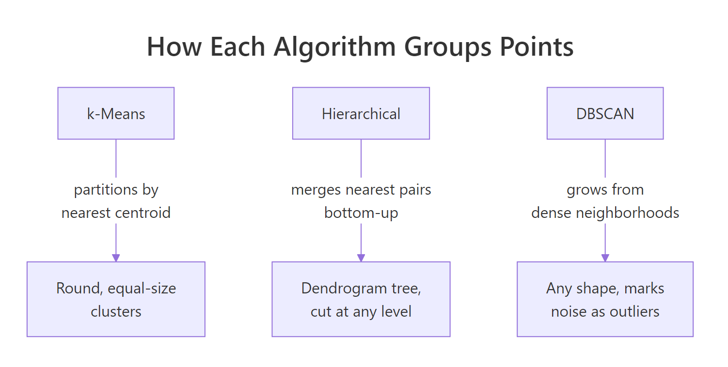
How each algorithm groups points differently.

Figure 1: How each algorithm groups points differently.

RFit k-Means with scaling and nstart

shapes_sc <- scale(shapes) # z-score each column km5 <- kmeans(shapes_sc, centers = 5, nstart = 25) km5 #> K-means clustering with 5 clusters of sizes 408, 196, 197, 100, 199 #> #> Within cluster sum of squares by cluster: #> [1] 92.1 32.5 35.8 18.4 41.7 #> (between_SS / total_SS = 88.7 %)

The between_SS / total_SS ratio, 88.7%, tells you how much of the total spread is explained by the cluster structure. Higher is tighter. This metric is useful when comparing two k-means fits with different k values on the same data.

RInspect centers and cluster sizes

km5$size # points per cluster #> [1] 408 196 197 100 199 round(km5$centers, 2) # cluster means in z-score space #> x y #> 1 0.52 0.21 #> 2 -1.14 -0.94 #> 3 -1.22 0.82 #> 4 1.68 1.21 #> 5 1.64 -0.94

The centers are in scaled units, so a value of 1.68 means "1.68 standard deviations above the mean on x". If you need centers in the original units, multiply back by the original column's standard deviation and add its mean, or call kmeans() on the raw (unscaled) data if columns share units.

Tip

Always set nstart = 25 or higher. The default of 1 gives the first random init, which can land in a poor local minimum. 25 takes milliseconds extra and gives you the best of 25 restarts.

Try it: Refit k-means on shapes_sc with centers = 3 and save as ex_km. Print ex_km$size to see the three new cluster sizes.

RYour turn: k-Means with k=3

ex_km <- NULL # ex_km$size #> Expected: three sizes summing to 1100

Click to reveal solution

Rk-Means k=3 solution

ex_km <- kmeans(shapes_sc, centers = 3, nstart = 25) ex_km$size #> [1] 405 496 199

Explanation: Going from k=5 to k=3 merges neighboring clusters. The total is still 1100 points because every point is partitioned.

How do you pick the right k with the elbow and silhouette?

For k-means and hierarchical, you pick k yourself. Two methods dominate in practice:

Elbow method (within-cluster sum of squares, WSS): plot WSS against k. The "elbow" is where adding another cluster stops buying you much compactness.
Silhouette width: plot the average silhouette against k. Pick the k that peaks. Silhouette measures how well each point sits inside its cluster versus the next nearest one.

fviz_nbclust() from factoextra runs the search and draws the plot in one call.

RElbow plot for optimal k

fviz_nbclust(shapes_sc, kmeans, method = "wss", nstart = 25) + labs(title = "Elbow method: WSS vs k")

Look for the point where the curve bends. On multishapes the bend sits around k=5 or k=6, which matches the five real shapes plus their overlaps.

RSilhouette plot for optimal k

fviz_nbclust(shapes_sc, kmeans, method = "silhouette", nstart = 25) + labs(title = "Silhouette method: avg width vs k")

Silhouette peaks where the within-cluster points are tight and the between-cluster separation is wide. A peak score above 0.5 is usually solid; below 0.25 means the clusters are not well separated and you should question whether clustering is the right tool.

Note

Elbow and silhouette can disagree. When they do, trust silhouette for compact clusters and WSS for elongated ones. If they disagree sharply, your data may not have a natural cluster structure.

Try it: Run fviz_nbclust() with method = "gap_stat" and save the plot as ex_gap. The gap statistic is a third optimizer that compares WSS against a null reference distribution.

RYour turn: gap statistic

set.seed(7) ex_gap <- NULL # ex_gap #> Expected: a ggplot showing the gap statistic against k

Click to reveal solution

RGap statistic solution

set.seed(7) ex_gap <- fviz_nbclust(shapes_sc, kmeans, method = "gap_stat", nboot = 50, nstart = 25) ex_gap

Explanation: The gap statistic runs 50 bootstrap resamples (nboot = 50) of uniformly distributed null data and compares the WSS gap. It's slower than the other two methods but often more robust on noisy data.

How does hierarchical clustering build a dendrogram?

Hierarchical clustering builds a tree, not a flat partition. It starts with every point as its own cluster, then repeatedly merges the two closest clusters until one cluster holds everything. The "closest" definition is called the linkage method, and it matters a lot.

The three linkages you'll meet in the wild:

Ward's ("ward.D2"), merges clusters that increase within-cluster variance the least. Tends to produce compact, round clusters. The default for most analyses.
Complete, merges based on the most distant pair of points between clusters. Produces tight, evenly sized clusters.
Single, merges based on the closest pair. Can produce long "chained" clusters that snake through the data.

Once the tree is built, you cut it at a chosen level with cutree() to get a flat cluster assignment.

RHierarchical clustering with Ward's linkage

d <- dist(shapes_sc) # pairwise distances hc <- hclust(d, method = "ward.D2") # build the tree hc_clusters <- cutree(hc, k = 5) # cut into 5 flat clusters table(hc_clusters) #> hc_clusters #> 1 2 3 4 5 #> 405 200 196 100 199

You get the tree once and can cut it at any k without refitting. That's one advantage over k-means, which must refit per k.

RPlot the dendrogram with k=5 highlighted

plot(hc, labels = FALSE, hang = -1, main = "Dendrogram (Ward's linkage)", xlab = "", sub = "") rect.hclust(hc, k = 5, border = 2:6)

Height on the y-axis is the linkage distance at which two clusters merge. The longer the vertical line between a merge and the next one below, the more distinct the clusters being joined. rect.hclust() draws boxes around the five groups that emerge at k=5.

Warning

Linkage choice changes the answer. Ward's and complete typically give similar results on compact data; single linkage can look nothing like either. Always state the linkage you used and, for important analyses, compare at least two.

Try it: Refit hierarchical clustering with method = "single" and cut at k=5. Save the cluster vector as ex_hc_single and compare its sizes with Ward's.

RYour turn: single linkage

ex_hc_single <- NULL # table(ex_hc_single) #> Expected: sizes very different from Ward's

Click to reveal solution

RSingle-linkage solution

hc_s <- hclust(d, method = "single") ex_hc_single <- cutree(hc_s, k = 5) table(ex_hc_single) #> ex_hc_single #> 1 2 3 4 5 #> 1096 1 1 1 1

Explanation: Single linkage put 1096 points into cluster 1 and made each of the other clusters a single point. This is the chaining effect: single linkage is happy to merge clusters via a single bridge point, collapsing everything into one giant group.

How does DBSCAN find clusters of arbitrary shape?

DBSCAN stands for Density-Based Spatial Clustering of Applications with Noise. Instead of a fixed k, it takes two parameters:

eps, the radius defining a point's neighborhood.
MinPts, the minimum number of neighbors within eps to call a point "core".

The algorithm then grows clusters by chaining together core points whose neighborhoods overlap. Points that don't fit into any cluster get label 0, meaning noise. This is why DBSCAN can handle concentric rings, crescents, and other shapes where every other algorithm fails, and it never forces outliers into a cluster they don't belong to.

The hard part is picking eps. A standard trick: plot the distance to each point's k-th nearest neighbor in ascending order. The "knee" in the curve, where the line bends sharply upward, is a good eps.

RPick eps with the kNN distance plot

kNNdistplot(shapes_sc, k = 5) abline(h = 0.15, lty = 2, col = "red") #> Look for the knee; the dashed line marks our choice of eps = 0.15

The dashed red line at eps = 0.15 sits right at the elbow of the curve, meaning most points have their 5th neighbor within 0.15 units and only the noise points reach beyond it. That's the sweet spot.

RFit DBSCAN with chosen parameters

db <- dbscan(shapes_sc, eps = 0.15, MinPts = 5) table(db$cluster) #> #> 0 1 2 3 4 5 #> 31 405 196 199 100 169

Cluster 0 contains the 31 noise points. The five real clusters (1 through 5) correspond to the five shapes in the dataset. Compare this to k-means, which forced those 31 outliers into cluster memberships they don't really belong to.

Key Insight

"Noise" is a feature, not a bug. In fraud detection, anomaly analysis, and quality control, the DBSCAN noise label is often exactly what you're looking for: points that don't fit any natural group. Treating them as cluster 0 keeps them out of downstream averages and models.

Try it: Refit DBSCAN on shapes_sc with eps = 0.5 (much larger). Save as ex_db and check table(ex_db$cluster). You'll see clusters merge.

RYour turn: bigger eps

ex_db <- NULL # table(ex_db$cluster) #> Expected: fewer clusters, fewer (or zero) noise points

Click to reveal solution

RDBSCAN with larger eps solution

ex_db <- dbscan(shapes_sc, eps = 0.5, MinPts = 5) table(ex_db$cluster) #> #> 0 1 #> 2 1098

Explanation: A too-large eps makes every point a neighbor of every other, so DBSCAN collapses everything into one giant cluster with almost no noise. This is why the kNN plot matters: it tells you the scale of "neighborhood" your data actually supports.

Which algorithm should you pick for your data?

After seeing all three in action, you now have the information you need to choose. The decision hinges on three questions: do you know k, are the clusters round, and do you need to handle outliers?

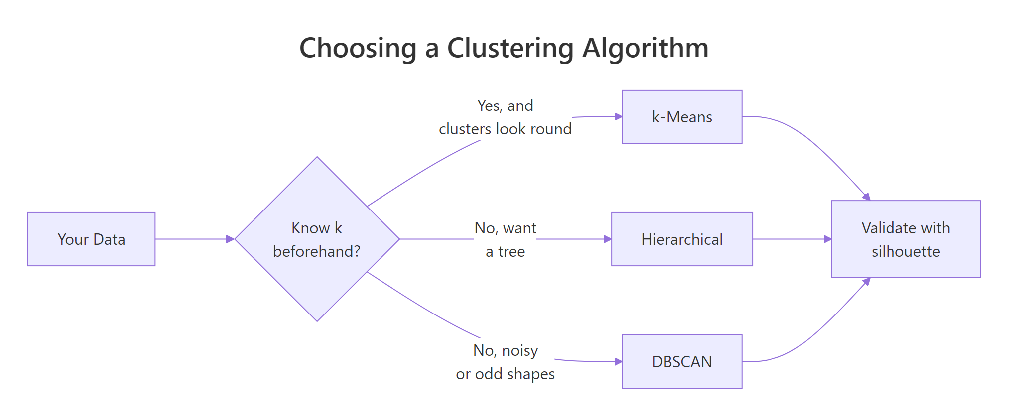
A quick decision path for picking a clustering algorithm.

Figure 2: A quick decision path for picking a clustering algorithm.

A compact guide:

Situation	Best pick	Why
You know k, clusters look round	k-Means	Fastest, simplest, scales to millions of rows
You want a tree to inspect	Hierarchical	Dendrogram reveals structure at every level
Shapes are irregular or you expect outliers	DBSCAN	Density-based, flags noise as cluster 0
Data has tens of millions of rows	k-Means	Others are O(n^2) in memory
You're exploring and don't know k	Hierarchical + silhouette	Tree + quantitative cut

For any clustering decision, the single most useful validation number is the average silhouette width. It ranges from -1 to 1: values above 0.5 are strong structure, 0.25 to 0.5 is weak but real, below 0.25 means the clustering may not be meaningful. Computing it on all three fits gives you an objective tiebreaker.

RCompare average silhouette width across all three algorithms

# Silhouette works on any cluster vector; needs distance matrix d_sc <- dist(shapes_sc) # k-means sil sil_km <- mean(silhouette(km5$cluster, d_sc)[, 3]) # hierarchical sil (cutree k=5) sil_hc <- mean(silhouette(cutree(hc, 5), d_sc)[, 3]) # dbscan sil (drop noise points, which have label 0) keep <- db$cluster != 0 sil_db <- mean(silhouette(db$cluster[keep], dist(shapes_sc[keep, ]))[, 3]) round(c(kmeans = sil_km, hierarchical = sil_hc, dbscan = sil_db), 3) #> kmeans hierarchical dbscan #> 0.418 0.425 0.613

DBSCAN wins with 0.613 because it ignored the noise points and only scored the density-coherent groups, exactly as it should. k-means and hierarchical paid the penalty for forcing outliers into the nearest cluster, which dragged their average silhouette down. When the shapes are irregular, DBSCAN dominates this benchmark; when they are round, k-means usually leads.

Tip

Run all three as a default audit. In 10 lines of R you can fit all three models and print their silhouette widths. That's cheaper than guessing wrong, and it often reveals structure a single algorithm would miss.

Try it: Compute the silhouette width for ex_km (your k=3 k-means fit) using d_sc and compare it to sil_km above.

RYour turn: silhouette for k=3

sil_ex <- NULL # sil_ex #> Expected: a single number between -1 and 1

Click to reveal solution

RSilhouette for k=3 solution

sil_ex <- mean(silhouette(ex_km$cluster, d_sc)[, 3]) round(sil_ex, 3) #> [1] 0.382

Explanation: k=3 on non-spherical shapes gives a lower silhouette (0.382) than k=5 (0.418), confirming that fewer clusters forced heterogeneous points together.

Practice Exercises

Exercise 1: k-Means on `iris`, does it match species?

Scale iris[, 1:4], run k-means with k = 3 and nstart = 25, then cross-tabulate the cluster against iris$Species. Save the cluster vector as my_km and the table as my_tbl.

RExercise 1 starter

# Hint: scale(), kmeans(), then table(clusters, iris$Species) # Write your code below:

Click to reveal solution

RExercise 1 solution

iris_sc <- scale(iris[, 1:4]) set.seed(42) my_km <- kmeans(iris_sc, centers = 3, nstart = 25)$cluster my_tbl <- table(cluster = my_km, species = iris$Species) my_tbl #> species #> cluster setosa versicolor virginica #> 1 50 0 0 #> 2 0 39 14 #> 3 0 11 36

Explanation: Cluster 1 is a perfect match for setosa. Clusters 2 and 3 mostly align with versicolor and virginica, with 25 misassignments where the two species overlap in petal space. Clustering is not a classifier, so this kind of partial alignment is normal.

Exercise 2: Hierarchical clustering of `USArrests`

Scale USArrests, run Ward's hierarchical clustering, cut at k = 4, and save the state-to-cluster mapping as my_states. Which cluster contains California?

RExercise 2 starter

# Hint: scale() -> dist() -> hclust(method='ward.D2') -> cutree(k=4) # Write your code below:

Click to reveal solution

RExercise 2 solution

us_sc <- scale(USArrests) my_hc <- hclust(dist(us_sc), method = "ward.D2") my_states <- cutree(my_hc, k = 4) my_states["California"] #> California #> 1 # Peek at the other states in California's cluster names(my_states[my_states == 1]) #> [1] "Arizona" "California" "Colorado" "Florida" "Illinois" #> [6] "Maryland" "Michigan" "Nevada" "New Mexico" "New York" #> [11] "Texas"

Explanation: California sits with 10 other high-crime, high-urbanization states. Ward's linkage groups states that are close in the combined space of murder, assault, rape, and urban population.

Exercise 3: k-Means vs DBSCAN on concentric rings

Generate two concentric rings with base R (inner ring radius 1, outer ring radius 3, both with small Gaussian noise). Save the 2-column matrix as my_rings. Fit kmeans(my_rings, 2) and dbscan(my_rings, eps = 0.3, MinPts = 5). Plot both colorings.

RExercise 3 starter

# Hint: use runif() for angles, then x = r*cos(theta), y = r*sin(theta) set.seed(1) n <- 300 # Write your code below:

Click to reveal solution

RExercise 3 solution

set.seed(1) n <- 300 t1 <- runif(n, 0, 2*pi); r1 <- 1 + rnorm(n, 0, 0.1) t2 <- runif(n, 0, 2*pi); r2 <- 3 + rnorm(n, 0, 0.1) my_rings <- rbind(cbind(r1*cos(t1), r1*sin(t1)), cbind(r2*cos(t2), r2*sin(t2))) my_km_r <- kmeans(my_rings, centers = 2, nstart = 25)$cluster my_db_r <- dbscan(my_rings, eps = 0.3, MinPts = 5)$cluster par(mfrow = c(1, 2)) plot(my_rings, col = my_km_r + 1, pch = 20, main = "k-Means on rings") plot(my_rings, col = my_db_r + 1, pch = 20, main = "DBSCAN on rings") par(mfrow = c(1, 1))

Explanation: k-Means cuts the rings in half because it can only draw straight boundaries between centroids. DBSCAN traces each ring cleanly because it follows density. This is the classic illustration of why algorithm choice matters more than tuning.

Complete Example: End-to-End on `iris`

Here is the full workflow from raw data to algorithm choice, applied to iris.

RComplete clustering workflow on iris

# 1. Prepare data (numeric columns only, scaled) iris_sc <- scale(iris[, 1:4]) # 2. Fit all three with k = 3 (we know there are 3 species) set.seed(123) iris_km <- kmeans(iris_sc, centers = 3, nstart = 25) iris_hc <- hclust(dist(iris_sc), method = "ward.D2") iris_db <- dbscan(iris_sc, eps = 0.9, MinPts = 5) # 3. Validate with average silhouette width d_iris <- dist(iris_sc) iris_sils <- c( kmeans = mean(silhouette(iris_km$cluster, d_iris)[, 3]), hierarchical = mean(silhouette(cutree(iris_hc, 3), d_iris)[, 3]), dbscan = mean(silhouette( iris_db$cluster[iris_db$cluster != 0], dist(iris_sc[iris_db$cluster != 0, ]))[, 3]) ) round(iris_sils, 3) #> kmeans hierarchical dbscan #> 0.460 0.446 0.605 # 4. Pick the winner for this dataset names(which.max(iris_sils)) #> [1] "dbscan"

DBSCAN wins on iris as well, but notice why: it discarded 17 noise points (the overlap zone between versicolor and virginica) and only scored the well-separated core. k-means and hierarchical had to classify those overlap points, which is harder. The lesson: the silhouette winner depends on whether you need every point assigned. If you do, k-means at 0.460 is your answer. If you don't, DBSCAN's 0.605 reflects tighter structure.

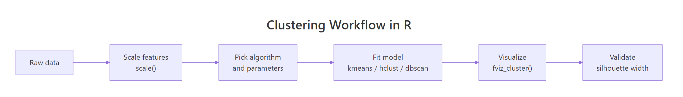
The end-to-end clustering workflow in R.

Figure 3: The end-to-end clustering workflow in R.

Summary

Algorithm	Function	Strength	Weakness	Best for
k-Means	`kmeans()`	Fast, scalable, simple	Assumes round clusters; needs k upfront	Large tabular data with roughly equal, compact groups
Hierarchical	`hclust()` + `cutree()`	Full tree at every k; interpretable	O(n²) memory; sensitive to linkage	Small-to-medium data where structure matters
DBSCAN	`dbscan::dbscan()`	Any shape; labels noise	Parameters eps/MinPts are finicky	Spatial data, anomaly detection, non-spherical clusters

Three recurring mistakes to avoid:

Clustering without scaling. Any algorithm using Euclidean distance is dominated by the column with the largest variance. Always scale() first unless columns share units.
Picking k without validation. fviz_nbclust() takes one line and will tell you if your k is defensible. Use it.
Ignoring DBSCAN because "it's for spatial data". DBSCAN works on any numeric matrix with meaningful distances. It's especially valuable when outliers matter.

References

Hastie, T., Tibshirani, R., & Friedman, J., The Elements of Statistical Learning, 2nd ed. (Springer, 2009), Chapter 14 on unsupervised learning. Link
factoextra package reference manual. Link
dbscan package on CRAN, Hahsler, M., Piekenbrock, M., Doran, D. Journal of Statistical Software 91(1), 2019. Link
Ester, M., Kriegel, H.-P., Sander, J., & Xu, X., A density-based algorithm for discovering clusters in large spatial databases with noise. KDD-96 Proceedings. Link
Ward, J. H., Hierarchical grouping to optimize an objective function. Journal of the American Statistical Association 58:236-244, 1963.
Rousseeuw, P. J., Silhouettes: a graphical aid to the interpretation and validation of cluster analysis. Journal of Computational and Applied Mathematics 20:53-65, 1987.
UC Business Analytics R Programming Guide, K-means and hierarchical clustering articles. Link
STHDA, DBSCAN for discovering clusters in data with noise. Link

Continue Learning

PCA in R, Reduce dimensions before clustering when your features are correlated.
Multivariate Distances, Understand the distance metrics that sit under every clustering algorithm.
Outlier Detection in R, DBSCAN's noise label is one approach; see the full toolkit for spotting anomalies.

Clustering in R: k-Means vs Hierarchical vs DBSCAN, How to Choose for Your Data

What happens when you run all three clustering algorithms on the same data?

How does k-Means partition data around centroids?

How do you pick the right k with the elbow and silhouette?

How does hierarchical clustering build a dendrogram?

How does DBSCAN find clusters of arbitrary shape?

Which algorithm should you pick for your data?

Practice Exercises

Exercise 1: k-Means on iris, does it match species?

Exercise 2: Hierarchical clustering of USArrests

Exercise 3: k-Means vs DBSCAN on concentric rings

Complete Example: End-to-End on iris

Summary

References

Continue Learning

Exercise 1: k-Means on `iris`, does it match species?

Exercise 2: Hierarchical clustering of `USArrests`

Complete Example: End-to-End on `iris`