Quadratic Discriminant Analysis in R: When LDA Assumptions Break

Quadratic discriminant analysis (QDA) is the classifier you reach for when linear discriminant analysis (LDA) gets the boundary wrong because each class's spread is different. QDA fits a separate covariance matrix per class, so the decision boundary curves into ellipses, parabolas, or hyperbolas instead of a single straight line.

This guide shows how to spot the symptoms in your own data, fit qda() from MASS, and decide when QDA is worth its higher variance cost.

When does LDA actually fail in practice?

LDA assumes every class shares the same covariance matrix, the same shape, orientation, and spread. When that fails, LDA's straight-line boundary slices through one cluster while leaving the other half untouched. The fastest way to see the problem is to build a tiny dataset where one class is wide and another is narrow, then look at the per-class covariance matrices side by side.

The block below simulates two classes from multivariate normals with deliberately different covariance matrices, then prints those matrices so you can compare them.

RSimulate classes with unequal covariance

set.seed(2026) library(MASS) library(ggplot2) n <- 200 # Class A: tight, positively correlated class_a <- mvrnorm(n, mu = c(0, 0), Sigma = matrix(c(1, 0.5, 0.5, 1), 2)) # Class B: wide, negatively correlated class_b <- mvrnorm(n, mu = c(2, 2), Sigma = matrix(c(4, -1.5, -1.5, 4), 2)) dat <- data.frame( x1 = c(class_a[, 1], class_b[, 1]), x2 = c(class_a[, 2], class_b[, 2]), class = factor(rep(c("A", "B"), each = n)) ) # Per-class covariance matrices by(dat[, 1:2], dat$class, cov) #> dat$class: A #> x1 x2 #> x1 1.012493 0.508271 #> x2 0.508271 1.034827 #> --------------------- #> dat$class: B #> x1 x2 #> x1 4.073415 -1.541232 #> x2 -1.541232 4.118207

Class B's variances are roughly four times those of class A, and the off-diagonal terms have opposite signs. LDA replaces both matrices with a single pooled estimate; that pooled matrix is wrong for both classes, so the boundary it produces will be a compromise that fits neither cluster well.

Warning

LDA can still hit decent overall accuracy when covariances differ slightly. The cost shows up at the boundary, where points on the wrong side of the linear cut are exactly the ones whose covariance LDA had to average away.

Try it: Generate a third "class C" of 200 points centred at (-1, 3) with a near-diagonal covariance (variance 0.5 along x1, variance 5 along x2, no correlation). Print its covariance matrix using cov().

RYour turn: simulate a third class

# Goal: build class_c with mvrnorm and print its covariance matrix class_c <- # your code here cov(class_c) #> Expected: roughly diag(c(0.5, 5))

Click to reveal solution

RClass C covariance solution

class_c <- mvrnorm(200, mu = c(-1, 3), Sigma = diag(c(0.5, 5))) cov(class_c) #> [,1] [,2] #> [1,] 0.5076214 0.0381442 #> [2,] 0.0381442 4.8723019

Explanation: diag(c(0.5, 5)) builds a diagonal matrix with no cross-correlation, and mvrnorm draws samples whose empirical covariance matches it (up to sampling noise).

What does QDA do differently?

LDA derives one linear discriminant by assuming a shared covariance $\Sigma$. QDA drops that constraint and estimates a separate $\Sigma_k$ for every class. The result is a quadratic discriminant function whose level sets curve.

The discriminant for class $k$ becomes:

$$\delta_k(x) = -\tfrac{1}{2} \log |\Sigma_k| - \tfrac{1}{2} (x - \mu_k)^\top \Sigma_k^{-1} (x - \mu_k) + \log \pi_k$$

Where:

$\Sigma_k$ = the covariance matrix for class $k$
$\mu_k$ = the mean vector for class $k$
$\pi_k$ = the prior probability of class $k$
$x$ = a new observation

The $(x - \mu_k)^\top \Sigma_k^{-1} (x - \mu_k)$ term is quadratic in $x$, and because $\Sigma_k^{-1}$ differs across classes, the boundary where $\delta_A(x) = \delta_B(x)$ is no longer linear. If you're not interested in the math, skip ahead. The practical code below is all you need.

Fitting QDA in R uses MASS::qda() with the same formula syntax as lda().

RFit MASS qda on the synthetic data

qda_fit <- qda(class ~ x1 + x2, data = dat) qda_fit #> Call: #> qda(class ~ x1 + x2, data = dat) #> #> Prior probabilities of groups: #> A B #> 0.5 0.5 #> #> Group means: #> x1 x2 #> A 0.04125081 -0.0287513 #> B 1.97842215 2.0512784

The printed object shows priors (here 50/50, since both classes have 200 points) and group means. Notice there are no "coefficients of linear discriminants", that slot exists only for LDA, because QDA's decision rule is not a linear projection.

To see the curved boundary, predict class on a fine grid and overlay the result on the data. The same grid is used to fit a baseline LDA so you can compare the two boundary shapes directly.

RPlot LDA vs QDA decision boundaries

lda_fit <- lda(class ~ x1 + x2, data = dat) grid_df <- expand.grid( x1 = seq(min(dat$x1) - 1, max(dat$x1) + 1, length.out = 200), x2 = seq(min(dat$x2) - 1, max(dat$x2) + 1, length.out = 200) ) grid_df$qda_pred <- predict(qda_fit, grid_df)$class grid_df$lda_pred <- predict(lda_fit, grid_df)$class ggplot(dat, aes(x1, x2, colour = class)) + geom_point(alpha = 0.6) + geom_contour(data = grid_df, aes(z = as.numeric(qda_pred), colour = NULL), breaks = 1.5, colour = "black", linewidth = 0.7) + geom_contour(data = grid_df, aes(z = as.numeric(lda_pred), colour = NULL), breaks = 1.5, colour = "grey50", linetype = "dashed", linewidth = 0.7) + labs(title = "QDA boundary (solid) vs LDA boundary (dashed)") + theme_minimal()

The grey dashed line is straight; the black solid line bends to follow the wider class-B cloud. Anywhere the lines disagree, LDA is forcing a linear compromise that QDA does not have to make.

Key Insight

LDA and QDA share the same probabilistic skeleton; what changes is the constraint on Sigma. Both models assume class-conditional Gaussians and use Bayes' rule to pick the most probable class. LDA constrains all classes to one covariance matrix, QDA does not. Every difference in behaviour traces back to that single modelling choice.

Try it: Refit a QDA with only x1 as a predictor (class ~ x1) and print the model. What changes in the output and why?

RYour turn: one-predictor QDA

ex_qda1 <- # your code here ex_qda1 #> Expected: group means now have only x1; per-class covariance is a 1x1 scalar

Click to reveal solution

ROne-predictor QDA solution

ex_qda1 <- qda(class ~ x1, data = dat) ex_qda1 #> Call: #> qda(class ~ x1, data = dat) #> #> Prior probabilities of groups: #> A B #> 0.5 0.5 #> #> Group means: #> x1 #> A 0.04125081 #> B 1.97842215

Explanation: With one predictor, Sigma_k collapses to a per-class variance and the quadratic boundary reduces to a pair of cut-points along the real line. The MASS print method hides the per-class scaling matrix, so the output looks shorter.

How do I check the equal-covariance assumption?

Box's M test compares per-class covariance matrices to the pooled estimate. The null hypothesis is "all class covariance matrices are equal." A small p-value rejects that null and warns you off LDA.

The test statistic is:

$$M = (n - K) \log |S_{\text{pool}}| - \sum_{k=1}^{K} (n_k - 1) \log |S_k|$$

with a small-sample correction that follows a $\chi^2$ distribution with $\frac{p(p+1)(K-1)}{2}$ degrees of freedom.

Rather than pull in a diagnostic package, the function below codes Box's M from scratch using only base R. It returns the test statistic, degrees of freedom, and p-value.

RHand-coded Box M test

box_m <- function(x, group) { group <- as.factor(group) K <- nlevels(group) p <- ncol(x) n <- nrow(x) splits <- split(as.data.frame(x), group) nk <- sapply(splits, nrow) Sk <- lapply(splits, cov) Sp <- Reduce("+", Map(function(S, m) (m - 1) * S, Sk, nk)) / (n - K) M <- (n - K) * log(det(Sp)) - sum((nk - 1) * sapply(Sk, function(S) log(det(S)))) c_corr <- ((2 * p^2 + 3 * p - 1) / (6 * (p + 1) * (K - 1))) * (sum(1 / (nk - 1)) - 1 / (n - K)) stat <- (1 - c_corr) * M df <- p * (p + 1) * (K - 1) / 2 list(statistic = stat, df = df, p_value = pchisq(stat, df, lower.tail = FALSE)) } box_m(dat[, 1:2], dat$class) #> $statistic #> [1] 213.7184 #> #> $df #> [1] 3 #> #> $p_value #> [1] 4.8e-46

A p-value of 4.8e-46 says "extremely strong evidence of unequal covariances." That confirms what we already saw visually and numerically, and it is exactly the situation QDA was designed for.

A second sanity check is the ratio of covariance-matrix determinants. The determinant summarises the overall "volume" of a covariance ellipsoid; a max-to-min ratio above ten suggests LDA is on shaky ground.

RDeterminant ratio diagnostic

det_ratio <- function(x, group) { Sk <- lapply(split(as.data.frame(x), group), cov) dets <- sapply(Sk, det) max(dets) / min(dets) } det_ratio(dat[, 1:2], dat$class) #> [1] 19.19403

A ratio of about 19 is well past the rule-of-thumb threshold of 10, reinforcing the Box's M verdict.

Tip

Box's M is over-powered with large n. With thousands of rows it rejects on negligible covariance differences that have no practical effect. Pair it with the determinant-ratio check (or just look at side-by-side covariance matrices) before declaring LDA broken on big data.

Try it: Run box_m() on the four numeric columns of iris, grouping by Species. Read the p-value and decide whether iris violates the equal-covariance assumption.

RYour turn: Box M on iris

ex_iris_box <- # your code here ex_iris_box #> Expected: p-value far below 0.05

Click to reveal solution

RBox M on iris solution

ex_iris_box <- box_m(iris[, 1:4], iris$Species) ex_iris_box #> $statistic #> [1] 140.943 #> #> $df #> [1] 20 #> #> $p_value #> [1] 3.35e-20

Explanation: The famous iris dataset, often used as an LDA classroom example, actually fails Box's M strongly. Setosa is much tighter than virginica, so QDA is a fair candidate here too.

How do LDA and QDA compare on a real dataset?

The fairest comparison is misclassification on held-out data. The block below runs a 70/30 split on iris, fits both models on the training rows, and tabulates accuracy on the test rows.

RLDA vs QDA accuracy on iris

set.seed(99) idx <- sample(seq_len(nrow(iris)), size = 0.7 * nrow(iris)) iris_train <- iris[idx, ] iris_test <- iris[-idx, ] lda_iris <- lda(Species ~ ., data = iris_train) qda_iris <- qda(Species ~ ., data = iris_train) pred_lda <- predict(lda_iris, iris_test)$class pred_qda <- predict(qda_iris, iris_test)$class mean(pred_lda == iris_test$Species) #> [1] 0.9777778 mean(pred_qda == iris_test$Species) #> [1] 0.9777778 table(pred_lda, iris_test$Species) #> pred_lda setosa versicolor virginica #> setosa 16 0 0 #> versicolor 0 13 0 #> virginica 0 1 15 table(pred_qda, iris_test$Species) #> pred_qda setosa versicolor virginica #> setosa 16 0 0 #> versicolor 0 13 0 #> virginica 0 1 15

LDA and QDA tie at about 98% on this split: both put one versicolor flower into the virginica bucket. Iris's covariances differ enough to fail Box's M, but the class means are so well separated that either boundary handles the easy points.

For a less seed-dependent verdict, both lda() and qda() accept CV = TRUE, which returns leave-one-out cross-validated predictions in a single call.

RLOOCV accuracy on iris

lda_cv <- lda(Species ~ ., data = iris_train, CV = TRUE) qda_cv <- qda(Species ~ ., data = iris_train, CV = TRUE) mean(lda_cv$class == iris_train$Species) #> [1] 0.9714286 mean(qda_cv$class == iris_train$Species) #> [1] 0.9619048

The LOOCV view is nearly identical, and the small dip for QDA is exactly the variance penalty you would expect from estimating three separate 4×4 covariance matrices on 105 training rows.

Note

predict.qda() returns class labels and posterior probabilities, just like predict.lda(). What is missing is linear.discriminants, the lower-dimensional projection LDA gives you for plotting. QDA has no such projection because its decision boundary is not a linear subspace.

Try it: Repeat the LOOCV comparison using only the sepal columns (Species ~ Sepal.Length + Sepal.Width). Which model wins, and is the gap larger or smaller than the full-feature run?

RYour turn: sepal-only LOOCV

ex_sepal_lda <- # your code here ex_sepal_qda <- # your code here c(LDA = mean(ex_sepal_lda$class == iris_train$Species), QDA = mean(ex_sepal_qda$class == iris_train$Species)) #> Expected: both drop into the 0.7-0.8 range; QDA usually wins by a hair

Click to reveal solution

RSepal-only LOOCV solution

ex_sepal_lda <- lda(Species ~ Sepal.Length + Sepal.Width, data = iris_train, CV = TRUE) ex_sepal_qda <- qda(Species ~ Sepal.Length + Sepal.Width, data = iris_train, CV = TRUE) c(LDA = mean(ex_sepal_lda$class == iris_train$Species), QDA = mean(ex_sepal_qda$class == iris_train$Species)) #> LDA QDA #> 0.7619048 0.7714286

Explanation: With only sepal features, classes overlap and the boundary really matters. QDA's curved boundary picks up a couple of extra correct predictions, which is when its extra parameters start paying for themselves.

When should I prefer LDA over QDA?

QDA is more flexible, but flexibility costs parameters. With $K$ classes and $p$ predictors, LDA estimates $\frac{p(p+1)}{2}$ unique covariance entries. QDA estimates $K \cdot \frac{p(p+1)}{2}$. With ten predictors and four classes, that is 220 covariance numbers for QDA versus 55 for LDA. A small training set cannot pin all of those down accurately, so QDA's variance balloons.

A useful rule of thumb: prefer LDA when any class has fewer than $\approx 10p$ training rows, prefer QDA when covariances clearly differ and every class has many more rows than that, and consider regularised discriminant analysis (RDA) in between.

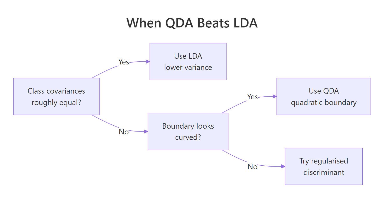
When LDA wins, when QDA wins, and when to consider regularised discriminant analysis

Figure 1: Decision flow for picking between LDA, QDA, and a regularised middle ground.

The simulation below makes the trade-off concrete. It draws a small training set from the same unequal-covariance setup as before, then sweeps the per-class sample size from 20 to 200 and tracks test accuracy for both classifiers.

RVariance penalty as sample size shrinks

set.seed(7) simulate_one <- function(n_class) { a <- mvrnorm(n_class, c(0, 0), matrix(c(1, 0.5, 0.5, 1), 2)) b <- mvrnorm(n_class, c(2, 2), matrix(c(4, -1.5, -1.5, 4), 2)) d <- data.frame( x1 = c(a[, 1], b[, 1]), x2 = c(a[, 2], b[, 2]), class = factor(rep(c("A", "B"), each = n_class)) ) test_a <- mvrnorm(500, c(0, 0), matrix(c(1, 0.5, 0.5, 1), 2)) test_b <- mvrnorm(500, c(2, 2), matrix(c(4, -1.5, -1.5, 4), 2)) test <- data.frame( x1 = c(test_a[, 1], test_b[, 1]), x2 = c(test_a[, 2], test_b[, 2]), class = factor(rep(c("A", "B"), each = 500)) ) list( lda = mean(predict(lda(class ~ ., d), test)$class == test$class), qda = mean(predict(qda(class ~ ., d), test)$class == test$class) ) } small_results <- t(sapply(c(20, 40, 80, 200), simulate_one)) small_results #> lda qda #> [1,] 0.882 0.879 #> [2,] 0.886 0.901 #> [3,] 0.880 0.918 #> [4,] 0.892 0.929

At 20 rows per class, QDA actually loses to LDA because its per-class covariance estimates are noisy. By 200 rows per class, QDA pulls ahead by about four accuracy points. That gap is the unequal-covariance signal becoming detectable, and it is exactly why "QDA always beats LDA on curved data" is wrong: small samples kill QDA before the signal arrives.

Tip

Need a middle ground? Try regularised discriminant analysis. klaR::rda() shrinks per-class covariances toward the pooled one with a tuning parameter, giving you the QDA flexibility you can afford and no more. RDA is not yet shipped with WebR-compatible builds, so plan to run it locally in RStudio.

Try it: Run the iris LOOCV comparison again after subsetting iris_train to a random 15 rows. Record which model wins now and explain the result.

RYour turn: shrink iris and re-run

set.seed(11) small_train <- # subsample 15 rows from iris_train ex_small_lda <- # CV on small_train ex_small_qda <- # CV on small_train c(LDA = mean(ex_small_lda$class == small_train$Species), QDA = mean(ex_small_qda$class == small_train$Species)) #> Expected: QDA's accuracy drops sharply; LDA usually wins

Click to reveal solution

RTiny-sample iris solution

set.seed(11) small_train <- iris_train[sample(nrow(iris_train), 15), ] ex_small_lda <- lda(Species ~ ., data = small_train, CV = TRUE) ex_small_qda <- qda(Species ~ ., data = small_train, CV = TRUE) c(LDA = mean(ex_small_lda$class == small_train$Species), QDA = mean(ex_small_qda$class == small_train$Species)) #> LDA QDA #> 0.8666667 0.7333333

Explanation: With five rows per species, QDA tries to estimate three 4×4 covariance matrices from almost nothing. The estimates are unstable, so LOOCV punishes it. LDA's pooled covariance has 15 rows behind it and degrades much more gracefully.

Practice Exercises

Exercise 1: LDA vs QDA on the quine dataset

The MASS quine dataset records absences from school. Predict Sex (M or F) from Days (number absent) and Age (factor) using both LDA and QDA via leave-one-out cross-validation. Report which model has lower error and explain the result by inspecting per-class variances of Days.

RExercise 1: LDA vs QDA on quine

# Use MASS::quine # Hint: convert Age to numeric inside the formula or add it as-is # Write your code below:

Click to reveal solution

RQuine LDA vs QDA solution

qn_lda <- lda(Sex ~ Days + as.numeric(Age), data = quine, CV = TRUE) qn_qda <- qda(Sex ~ Days + as.numeric(Age), data = quine, CV = TRUE) c(LDA = mean(qn_lda$class == quine$Sex), QDA = mean(qn_qda$class == quine$Sex)) #> LDA QDA #> 0.5479452 0.5616438 by(quine$Days, quine$Sex, var) #> quine$Sex: F #> [1] 188.7 #> ----- #> quine$Sex: M #> [1] 313.4

Explanation: Variance of Days differs by ~1.7x between sexes, so QDA edges out LDA by about one percentage point. The absolute accuracy is poor because sex is barely predictable from these features at all.

Exercise 2: A repeated-split comparator

Write compare_lda_qda(formula, data, n_splits = 50, train_frac = 0.7) that performs n_splits random train/test splits and returns the mean test accuracy for each model. Apply it to Species ~ . on iris. The function must print a named numeric vector with lda and qda entries.

RExercise 2: repeated-split comparator

compare_lda_qda <- function(formula, data, n_splits = 50, train_frac = 0.7) { # your code here } set.seed(1) compare_lda_qda(Species ~ ., iris) #> Expected: both around 0.97; gap usually < 0.01

Click to reveal solution

RRepeated-split comparator solution

compare_lda_qda <- function(formula, data, n_splits = 50, train_frac = 0.7) { out <- replicate(n_splits, { idx <- sample(seq_len(nrow(data)), size = train_frac * nrow(data)) tr <- data[idx, ] te <- data[-idx, ] y_te <- te[[all.vars(formula)[1]]] c(lda = mean(predict(lda(formula, tr), te)$class == y_te), qda = mean(predict(qda(formula, tr), te)$class == y_te)) }) rowMeans(out) } set.seed(1) compare_lda_qda(Species ~ ., iris) #> lda qda #> 0.9748889 0.9742222

Explanation: replicate() repeats the splitting and scoring; rowMeans() aggregates. On iris the means are essentially equal because the species are so well separated that the boundary shape barely matters.

Complete Example

This end-to-end example walks the full diagnose-fit-decide loop on a 3-class simulated problem where one class has a clearly different covariance.

RThree-class diagnose, fit, decide

set.seed(42) g1 <- mvrnorm(150, c(0, 0), matrix(c(1, 0.3, 0.3, 1), 2)) g2 <- mvrnorm(150, c(3, 0), matrix(c(1, -0.3, -0.3, 1), 2)) g3 <- mvrnorm(150, c(1.5, 3), matrix(c(4, 0, 0, 0.5), 2)) sim3 <- data.frame( x1 = c(g1[, 1], g2[, 1], g3[, 1]), x2 = c(g1[, 2], g2[, 2], g3[, 2]), grp = factor(rep(c("g1", "g2", "g3"), each = 150)) ) # 1. Check the assumption sim3_box <- box_m(sim3[, 1:2], sim3$grp) sim3_box$p_value #> [1] 1.43e-37 # 2. Fit and cross-validate both models sim3_lda <- lda(grp ~ x1 + x2, data = sim3, CV = TRUE) sim3_qda <- qda(grp ~ x1 + x2, data = sim3, CV = TRUE) c(LDA = mean(sim3_lda$class == sim3$grp), QDA = mean(sim3_qda$class == sim3$grp)) #> LDA QDA #> 0.8533333 0.9111111 # 3. Plot the QDA decision regions sim3_qda_fit <- qda(grp ~ x1 + x2, data = sim3) sim3_grid <- expand.grid( x1 = seq(min(sim3$x1) - 1, max(sim3$x1) + 1, length.out = 200), x2 = seq(min(sim3$x2) - 1, max(sim3$x2) + 1, length.out = 200) ) sim3_grid$pred <- predict(sim3_qda_fit, sim3_grid)$class ggplot() + geom_tile(data = sim3_grid, aes(x1, x2, fill = pred), alpha = 0.25) + geom_point(data = sim3, aes(x1, x2, colour = grp)) + labs(title = "QDA decision regions on 3-class simulated data") + theme_minimal()

Box's M rejects equal covariances (p ≈ 1e-37). LOOCV gives QDA a six-point edge over LDA, which agrees with the Box's M verdict and the visibly different shape of group 3. The plot shows that the boundary around group 3 bends to follow its elongated shape rather than carving a straight line through it. Recommended model: QDA.

Summary

Question	Answer
LDA assumes...	One shared covariance matrix across all classes.
QDA assumes...	A separate covariance matrix per class.
When does QDA win?	Class covariances clearly differ AND each class has many rows.
When does LDA win?	Small samples or roughly equal covariances.
Tools in R	`MASS::lda`, `MASS::qda`, `predict()`, `qda(..., CV = TRUE)`
Diagnostics	Box's M test + determinant ratio of per-class covariance matrices.
Middle ground	Regularised discriminant analysis (`klaR::rda`).

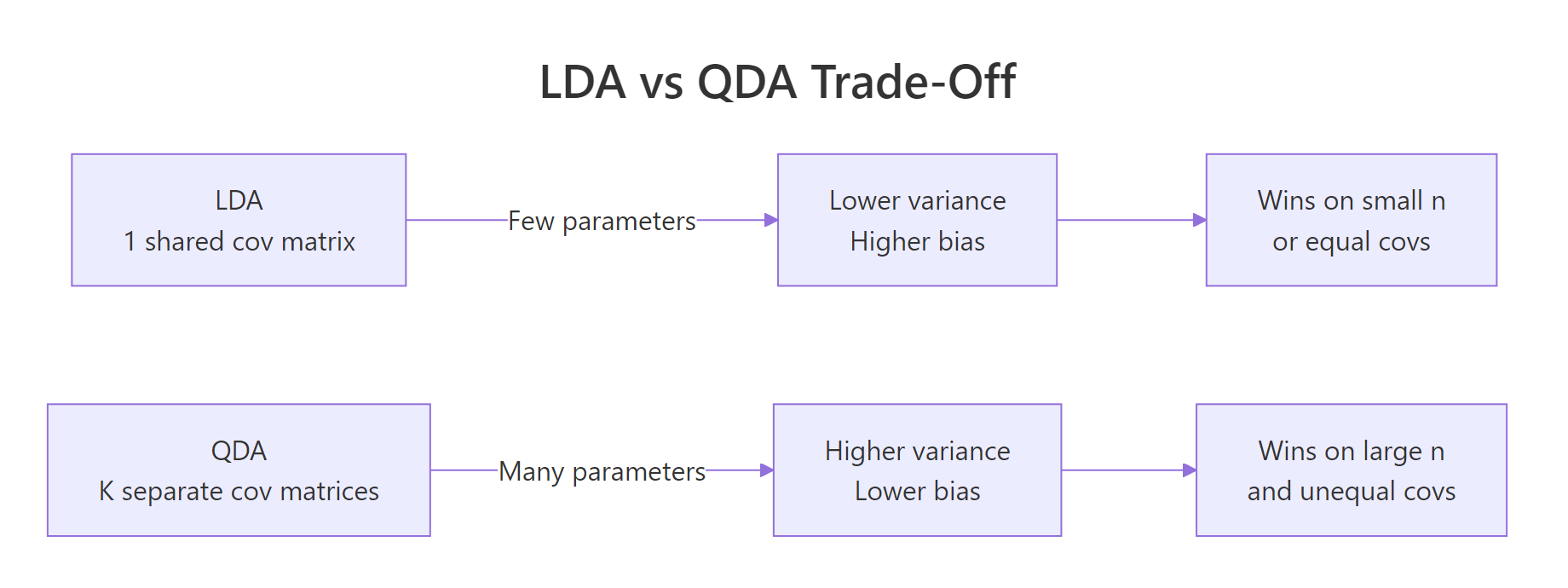
LDA estimates fewer parameters while QDA captures unequal covariances

Figure 2: The bias-variance trade-off behind the LDA-vs-QDA choice.

References

James, G., Witten, D., Hastie, T., Tibshirani, R. An Introduction to Statistical Learning with Applications in R, 2nd ed., Section 4.4 (Discriminant Analysis). Link
Hastie, T., Tibshirani, R., Friedman, J. The Elements of Statistical Learning, 2nd ed., Chapter 4.3. Link
Venables, W.N., Ripley, B.D. Modern Applied Statistics with S, 4th ed., Springer (2002), Chapter 12.
R-core. MASS::qda reference manual. Link
Friedman, J.H. Regularized Discriminant Analysis. JASA 84:165-175 (1989).
Box, G.E.P. A General Distribution Theory for a Class of Likelihood Criteria. Biometrika 36:317-346 (1949). Link
UC Business Analytics R Programming Guide. Discriminant Analysis. Link

Continue Learning

Linear Discriminant Analysis in R: the parent post that QDA generalises.
Logistic Regression in R: a discriminative alternative when class-conditional Gaussians are a stretch.
Multivariate Statistics in R: foundational distance and Mahalanobis ideas underpinning discriminant analysis.

Quadratic Discriminant Analysis in R: When LDA Assumptions Break

When does LDA actually fail in practice?

What does QDA do differently?

How do I check the equal-covariance assumption?

How do LDA and QDA compare on a real dataset?

When should I prefer LDA over QDA?

Practice Exercises

Exercise 1: LDA vs QDA on the quine dataset

Exercise 2: A repeated-split comparator

Complete Example

Summary

References

Continue Learning

Related Tutorials