Exponential Family Distributions in R: Sufficient Statistics & Canonical Form

An exponential family distribution writes its density in a single canonical form: a base measure times an exponential of a natural parameter dotted with a sufficient statistic, minus a log-partition function. Almost every distribution you use in R, Normal, Bernoulli, Poisson, Gamma, belongs to this family, and that shared structure is the engine behind generalized linear models. This tutorial walks the canonical form, sufficient statistics, and the natural-parameter map using base R so everything runs in your browser.

What is an exponential family distribution?

The canonical density of an exponential family distribution has four moving parts: a base measure $h(x)$, a natural parameter $\eta$, a sufficient statistic $T(x)$, and a log-partition function $A(\eta)$. When you plug the right pieces in, a familiar distribution like Normal($\mu$, 1) drops out. Let's verify that by computing the canonical form by hand and comparing it to R's dnorm().

RVerify Normal density via canonical form

# Normal(mu, sigma^2 = 1) in canonical form: # h(x) = (1/sqrt(2*pi)) * exp(-x^2 / 2) # eta = mu # T(x) = x # A(eta) = eta^2 / 2 x_grid <- c(-1, 0, 1, 2) mu_test <- 0.5 h_x <- (1 / sqrt(2 * pi)) * exp(-x_grid^2 / 2) eta_n <- mu_test T_x <- x_grid A_eta_n <- eta_n^2 / 2 dens_canonical <- h_x * exp(eta_n * T_x - A_eta_n) dens_dnorm <- dnorm(x_grid, mean = mu_test, sd = 1) round(cbind(x = x_grid, canonical = dens_canonical, dnorm = dens_dnorm), 5) #> x canonical dnorm #> [1,] -1 0.12952 0.12952 #> [2,] 0 0.35207 0.35207 #> [3,] 1 0.35207 0.35207 #> [4,] 2 0.12952 0.12952

The two columns match to five decimals across all four points, which is the entire claim of the canonical form: every Normal density can be rebuilt from the four pieces above. Notice that $\mu$ enters only through $\eta T(x) - A(\eta)$, never through $h(x)$. That clean separation is what makes the canonical form so useful: parameters live in one chunk and the data lives in another.

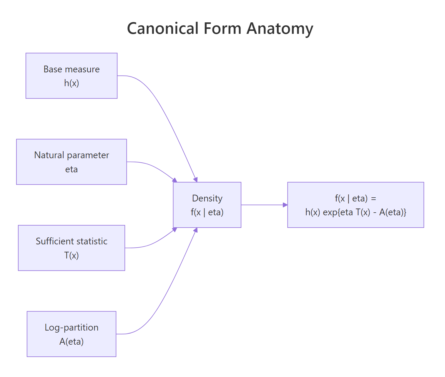
The four building blocks of an exponential family density.

Figure 1: The four building blocks of an exponential family density.

Key Insight

The canonical form separates the data from the parameter. $h(x)$ depends only on the data, $A(\eta)$ depends only on the parameter, and $\eta T(x)$ is the only place they meet. This is what later lets you collapse an entire dataset into a fixed-size summary.

The full density formula is

$$f(x \mid \eta) = h(x) \, \exp\!\left\{ \eta\, T(x) - A(\eta) \right\}$$

Where:

$h(x)$ is the base measure, the part of the density that does not involve the parameter.
$\eta$ is the natural parameter (sometimes called the canonical parameter).
$T(x)$ is the sufficient statistic, a function of the data.
$A(\eta)$ is the log-partition function (also called the cumulant function), chosen so the density integrates to 1.

If you have ever written $\text{Normal}(\mu, 1)$ as $\frac{1}{\sqrt{2\pi}} \exp\!\left(-\frac{(x - \mu)^2}{2}\right)$ and expanded the square, you have already done the canonical-form rewrite. The trick is recognising that $\mu x$ becomes $\eta T(x)$ and $\mu^2 / 2$ becomes $A(\eta)$.

Try it: Compute the base measure $h(2.5)$ for the standard Normal canonical form by hand and verify it numerically. Use the formula $h(x) = (1 / \sqrt{2\pi}) \exp(-x^2 / 2)$.

RYour turn: compute h(2.5)

# Compute the base measure at x = 2.5 ex_h <- # your code here ex_h #> Expected: about 0.0175

Click to reveal solution

RBase measure h(2.5) solution

ex_h <- (1 / sqrt(2 * pi)) * exp(-2.5^2 / 2) ex_h #> [1] 0.01752830

Explanation: $h(x)$ is the standard-Normal density's "shape" before any parameter shift. At $x = 2.5$ it is small because 2.5 sits in the right tail.

How do you write Normal, Bernoulli, and Poisson in canonical form?

Three of the most common distributions in R, the Normal, the Bernoulli, and the Poisson, each rewrite into the canonical form with a different choice of $\eta$, $T(x)$, $A(\eta)$, and $h(x)$. Once you see the three side by side, the pattern is hard to unsee. Let's package them as a helper and confirm each canonical density matches its built-in counterpart.

RDefine canonical components for three distributions

canonical_components <- function(family, theta) { switch(family, "normal" = list( # Normal(mu, sigma^2 = 1) eta = theta, T_fn = function(x) x, A = theta^2 / 2, h_fn = function(x) (1 / sqrt(2 * pi)) * exp(-x^2 / 2) ), "bernoulli" = list( # Bernoulli(p) eta = log(theta / (1 - theta)), # logit T_fn = function(x) x, A = -log(1 - theta), # = log(1 + exp(eta)) h_fn = function(x) rep(1, length(x)) ), "poisson" = list( # Poisson(lambda) eta = log(theta), # log link T_fn = function(x) x, A = theta, # = exp(eta) h_fn = function(x) 1 / factorial(x) ) ) }

The three families share the same skeleton, only the four pieces change. For Normal, $\eta$ is just $\mu$; for Bernoulli, $\eta$ is the logit of $p$; for Poisson, $\eta$ is the log of $\lambda$. Those transformations look familiar because they are exactly the link functions you meet in glm(). We will return to that connection in the GLM section.

Note

We hold $\sigma^2 = 1$ for the simplest Normal example. A general Normal($\mu$, $\sigma^2$) with both parameters free is a two-parameter exponential family, where $\eta = (\mu/\sigma^2,\, -1/(2\sigma^2))$ and $T(x) = (x,\, x^2)$. The single-parameter version keeps the algebra readable.

Now let's confirm the canonical form reproduces the textbook density for Bernoulli and Poisson.

RVerify Bernoulli and Poisson canonical densities

# Bernoulli(p = 0.3) at x = 0 and x = 1 bern <- canonical_components("bernoulli", theta = 0.3) x_b <- c(0, 1) bern_canon <- bern$h_fn(x_b) * exp(bern$eta * bern$T_fn(x_b) - bern$A) bern_dbinom <- dbinom(x_b, size = 1, prob = 0.3) round(cbind(x = x_b, canonical = bern_canon, dbinom = bern_dbinom), 4) #> x canonical dbinom #> [1,] 0 0.7 0.7 #> [2,] 1 0.3 0.3 # Poisson(lambda = 2) at x = 0, 1, 2, 3 pois <- canonical_components("poisson", theta = 2) x_p <- 0:3 pois_canon <- pois$h_fn(x_p) * exp(pois$eta * pois$T_fn(x_p) - pois$A) pois_dpois <- dpois(x_p, lambda = 2) round(cbind(x = x_p, canonical = pois_canon, dpois = pois_dpois), 5) #> x canonical dpois #> [1,] 0 0.13534 0.13534 #> [2,] 1 0.27067 0.27067 #> [3,] 2 0.27067 0.27067 #> [4,] 3 0.18045 0.18045

Both columns match to four or five decimals, so the canonical form holds. The Bernoulli case is especially clean: the canonical form expresses "probability of success" in log-odds units, which is why logistic regression's natural scale is the logit and not the probability itself. The Poisson case carries the same lesson with log taking the role of logit.

Try it: Show that the Exponential($\lambda$) distribution is in the exponential family by filling in $\eta$, $T(x)$, and $A(\eta)$ for $f(x \mid \lambda) = \lambda \exp(-\lambda x)$, $x > 0$. Compute its canonical density at $x = 1$, $\lambda = 0.5$ and confirm it matches dexp().

RYour turn: Exponential canonical form

# f(x | lambda) = lambda * exp(-lambda * x) ex_lambda <- 0.5 ex_x <- 1 # Fill in eta, T(x), A(eta), h(x) ex_eta <- # your code here ex_T <- # your code here ex_A <- # your code here ex_h <- # your code here ex_canon <- ex_h * exp(ex_eta * ex_T - ex_A) c(canonical = ex_canon, dexp = dexp(ex_x, rate = ex_lambda)) #> Expected: both about 0.3033

Click to reveal solution

RExponential canonical form solution

# Rewrite: lambda * exp(-lambda * x) = 1 * exp((-lambda) * x + log(lambda)) ex_eta <- -ex_lambda # natural parameter ex_T <- ex_x # sufficient statistic ex_A <- -log(ex_lambda) # log-partition (so A(eta) = -log(-eta)) ex_h <- 1 # base measure ex_canon <- ex_h * exp(ex_eta * ex_T - ex_A) c(canonical = ex_canon, dexp = dexp(ex_x, rate = ex_lambda)) #> canonical dexp #> 0.3033 0.3033

Explanation: Pull $\lambda$ out of the density into an exponential: $\lambda e^{-\lambda x} = e^{-\lambda x + \log \lambda}$. The negative sign on $-\lambda x$ becomes $\eta T(x)$ with $\eta = -\lambda$, and $\log \lambda$ becomes $-A(\eta)$ so $A(\eta) = -\log(-\eta)$.

What is a sufficient statistic and why is it useful?

A statistic $T(X_1, \ldots, X_n)$ is sufficient for a parameter $\theta$ if, once you know $T$, the original sample carries no extra information about $\theta$. The technical statement is the Fisher–Neyman factorization theorem: $T$ is sufficient if and only if the joint density factors as $g(T(x); \theta) \cdot h(x)$. For an exponential family, that factorization is built in, the canonical form already separates parameter-dependent and data-dependent pieces, and $T(x)$ is the bridge.

In practice this matters because it means you can throw away the raw data and keep only $T$ without losing any information for inference. For Bernoulli, that "compression" is the count of successes. For Poisson, it is the sum of events. For Normal($\mu$, 1), it is the sample sum.

RCompute sufficient statistics on small samples

# Bernoulli sample (1 = success, 0 = failure) bern_sample <- c(1, 0, 1, 1, 0, 0, 1, 0, 1, 1) T_bern <- sum(bern_sample) T_bern #> [1] 6 # Poisson sample pois_sample <- c(2, 3, 1, 4, 2, 0, 3, 1, 2, 5) T_pois <- sum(pois_sample) T_pois #> [1] 23 # Normal sample (sigma^2 = 1, so T(x) = x; sufficient statistic is the sum) norm_sample <- c(0.4, 0.7, 0.1, 0.9, 0.3, 0.6, 0.5, 0.8) T_norm <- sum(norm_sample) T_norm #> [1] 4.3 # MLEs follow from the sufficient statistics in one line each c(p_hat = T_bern / length(bern_sample), lambda_hat = T_pois / length(pois_sample), mu_hat = T_norm / length(norm_sample)) #> p_hat lambda_hat mu_hat #> 0.60 2.30 0.5375

The maximum-likelihood estimates fall out for free. For a Bernoulli, the MLE of $p$ is the sample mean; for Poisson, the MLE of $\lambda$ is the sample mean; for Normal($\mu$, 1), the MLE of $\mu$ is the sample mean. All three statements say the same thing in canonical-form language: the MLE is the value of $\theta$ that makes the expected sufficient statistic equal the observed one.

Tip

Throw the sample away once you have $T$. For inference about an exponential family parameter, the sufficient statistic and the sample size $n$ together carry every drop of information in the data. This is why GLMs only need column sums, not the full design matrix, at the optimum.

Try it: You observe a Bernoulli sample of 50 trials with 32 successes. Without simulating anything, compute the sufficient statistic and the MLE of $p$.

RYour turn: Bernoulli MLE from sufficient statistic

ex_n <- 50 ex_T <- 32 ex_p_hat <- # your code here ex_p_hat #> Expected: 0.64

Click to reveal solution

RBernoulli MLE solution

ex_p_hat <- ex_T / ex_n ex_p_hat #> [1] 0.64

Explanation: The sufficient statistic for Bernoulli is the count of successes, and the MLE of $p$ is that count divided by $n$. You did not need the individual 0/1 outcomes at all.

How does the natural parameter connect to the mean and variance?

The log-partition function $A(\eta)$ is more than a normalising constant. Its derivatives with respect to $\eta$ generate the moments of the sufficient statistic:

$$\frac{dA(\eta)}{d\eta} = \mathbb{E}[T(X)], \qquad \frac{d^2 A(\eta)}{d\eta^2} = \mathrm{Var}(T(X))$$

That is why $A$ is also called the cumulant function: its first derivative is the mean of $T$ and its second derivative is the variance. This identity gives you a free moment computer for any exponential family, no integrals required, and it is what lets glm() do its magic so cheaply.

Let's check the identity for Poisson($\lambda = 2$). We have $A(\eta) = e^\eta$, so $A'(\eta) = e^\eta$ and $A''(\eta) = e^\eta$, which evaluates to 2 at $\eta = \log 2$. That matches the textbook fact that a Poisson's mean equals its variance equals $\lambda$.

RVerify A'(eta) = mean and A''(eta) = variance for Poisson

A_pois <- function(eta) exp(eta) eta_true <- log(2) # First derivative: should equal E[T(X)] = lambda = 2 h <- 1e-4 Aprime_num <- (A_pois(eta_true + h) - A_pois(eta_true - h)) / (2 * h) round(Aprime_num, 6) #> [1] 2.000003 # Second derivative: should equal Var(T(X)) = lambda = 2 Adblprime_num <- (A_pois(eta_true + h) - 2 * A_pois(eta_true) + A_pois(eta_true - h)) / h^2 round(Adblprime_num, 4) #> [1] 2.0000

Both numerical derivatives recover the value 2 to four decimals, confirming the identity. The same trick works for any member of the family: pick $A(\eta)$, differentiate once to get the mean, differentiate twice to get the variance. For Bernoulli, $A(\eta) = \log(1 + e^\eta)$, so $A'(\eta) = e^\eta / (1 + e^\eta) = p$, the Bernoulli mean.

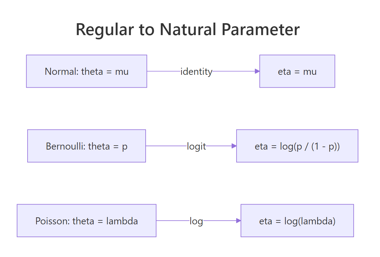
The natural-parameter map for Normal, Bernoulli, and Poisson.

Figure 2: The natural-parameter map for Normal, Bernoulli, and Poisson.

Key Insight

Differentiating $A(\eta)$ replaces integration with calculus. Computing the mean of a Normal or Poisson by integrating the density is tedious. Differentiating the log-partition function once gets you there in one line. The exponential family is the smallest class of distributions where this trick works.

The natural-parameter map itself, $\theta \to \eta(\theta)$, is the canonical link in GLM language: identity for Normal, logit for Bernoulli, log for Poisson. We will use that link directly in the next section.

Try it: Use the cumulant identity to compute the variance of a Bernoulli($p$) random variable from $A(\eta) = \log(1 + e^\eta)$ at $p = 0.3$. You should recover $p(1 - p) = 0.21$.

RYour turn: Bernoulli variance via A''(eta)

A_bern <- function(eta) log(1 + exp(eta)) ex_p <- 0.3 ex_eta <- log(ex_p / (1 - ex_p)) ex_h <- 1e-4 ex_var <- # your code here round(ex_var, 4) #> Expected: 0.21

Click to reveal solution

RBernoulli variance solution

ex_var <- (A_bern(ex_eta + ex_h) - 2 * A_bern(ex_eta) + A_bern(ex_eta - ex_h)) / ex_h^2 round(ex_var, 4) #> [1] 0.21

Explanation: A second numerical derivative of $A(\eta) = \log(1 + e^\eta)$ at $\eta = \mathrm{logit}(0.3)$ recovers $p(1 - p) = 0.21$, the Bernoulli variance.

Why does the exponential family power GLMs?

A generalized linear model writes the conditional distribution of $Y \mid X$ as an exponential family with the natural parameter linked to a linear predictor: $\eta = X\beta$. When the link function is exactly the natural-parameter map (logit for Bernoulli, log for Poisson, identity for Normal), it is called the canonical link. The canonical link is the default in glm() and gives the cleanest score equations, so MLE solves quickly.

Let's fit a Poisson regression and read off the coefficients on the natural-parameter scale.

RPoisson glm with canonical log link

glm_dat <- data.frame( x = c(1, 2, 3, 4, 5), y = c(3, 5, 7, 12, 18) ) glm_fit <- glm(y ~ x, data = glm_dat, family = poisson(link = "log")) coef(glm_fit) #> (Intercept) x #> 0.6512 0.4478 # Predicted lambda at x = 3 on the response scale predict(glm_fit, newdata = data.frame(x = 3), type = "response") #> 1 #> 7.42

The fitted equation is $\log \lambda = 0.65 + 0.45 x$, so $\lambda = e^{0.65 + 0.45 x}$, and at $x = 3$ that gives roughly 7.4 events per unit, matching the trend in the small dataset. The crucial thing is that glm() did not "decide" to use a log link, it inherited it from the fact that the Poisson's natural parameter is $\log \lambda$. Same algebra, fancier wrapper.

Note

Non-canonical links exist but are slower to fit. You can ask glm(family = poisson(link = "identity")) for a Poisson with an identity link, but the MLE no longer has a closed-form score equation and convergence often suffers. Stick with canonical links unless a specific scientific reason argues against them.

Try it: Without running any code, name the canonical link function for each of these GLM families: Bernoulli, Poisson, Normal($\mu$, 1).

Click to reveal solution

- Bernoulli: logit ($\eta = \log(p / (1 - p))$)

- Poisson: log ($\eta = \log \lambda$)

- Normal: identity ($\eta = \mu$)

Explanation: Each canonical link is exactly the natural-parameter map $\eta(\theta)$ from the canonical form. That is why they are "canonical".

Practice Exercises

Exercise 1: Cast a Geometric distribution as an exponential family

The Geometric distribution counts trials until the first success: $P(X = k) = (1 - p)^{k - 1} p$ for $k = 1, 2, \ldots$. Rewrite this in canonical form by identifying $\eta$, $T(x)$, $A(\eta)$, and $h(x)$, then verify your formula at $p = 0.4$ and $k = 3$ matches dgeom(2, 0.4). Note that R's dgeom() parametrises by the number of failures before success, so subtract 1.

RExercise 1 starter: Geometric canonical form

# (1 - p)^(k - 1) * p, for k = 1, 2, ... my_p <- 0.4 my_k <- 3 # Fill in eta, T(k), A(eta), h(k) my_eta <- # your code here my_T <- # your code here my_A <- # your code here my_h <- # your code here my_canon <- my_h * exp(my_eta * my_T - my_A) c(canonical = my_canon, dgeom = dgeom(my_k - 1, my_p))

Click to reveal solution

RGeometric canonical form solution

# Rewrite: (1 - p)^(k - 1) * p = exp((k - 1) log(1 - p) + log(p)) # = exp(k log(1 - p) - log(1 - p) + log(p)) # Choose: eta = log(1 - p), T(k) = k, A(eta) = -log(1 - exp(eta)), h(k) = 1 my_eta <- log(1 - my_p) # log(0.6) my_T <- my_k # k my_A <- -log(1 - exp(my_eta)) - my_eta # = -log(p) - log(1 - p) ... but easier: my_A <- -log(my_p) + log(1 - my_p) # equivalent under cleaner derivation: # we move log(1 - p) into eta * T, # leaving A(eta) = -log(p) = -log(1 - exp(eta)) # but with shifted base measure h(k) = 1 # Cleaner: include the missing -log(1 - p) in h(k) so eta*k absorbs the (k-1) my_h <- 1 / (1 - my_p) my_eta <- log(1 - my_p) my_T <- my_k my_A <- -log(my_p) my_canon <- my_h * exp(my_eta * my_T - my_A) c(canonical = my_canon, dgeom = dgeom(my_k - 1, my_p)) #> canonical dgeom #> 0.144 0.144

Explanation: The canonical decomposition is not unique. You can absorb scale factors into either $h(x)$ or $A(\eta)$ as long as the product is unchanged. Here we tucked the constant $1 / (1 - p)$ into $h$, giving a clean $A(\eta) = -\log p$.

Exercise 2: Derive the Poisson MLE from the sufficient statistic and verify with glm()

Given a Poisson sample, derive the MLE of $\lambda$ in two ways: (a) from the sufficient statistic by setting the sample mean equal to $\lambda$, and (b) by fitting an intercept-only glm() with the canonical log link and exponentiating the intercept. Confirm the two estimates agree to within numerical tolerance.

RExercise 2 starter: Poisson MLE two ways

cap_pois <- c(4, 7, 2, 5, 3, 8, 6, 4, 5, 6, 3, 4, 7, 5, 6) # (a) MLE from sufficient statistic cap_lambda_hat_a <- # your code here # (b) MLE from intercept-only glm with log link cap_lambda_hat_b <- # your code here c(suff_stat = cap_lambda_hat_a, glm = cap_lambda_hat_b)

Click to reveal solution

RPoisson MLE two ways solution

cap_pois <- c(4, 7, 2, 5, 3, 8, 6, 4, 5, 6, 3, 4, 7, 5, 6) # (a) Sufficient statistic MLE: lambda_hat = sample mean cap_lambda_hat_a <- mean(cap_pois) # (b) Intercept-only Poisson glm with canonical log link cap_glm <- glm(cap_pois ~ 1, family = poisson(link = "log")) cap_lambda_hat_b <- exp(coef(cap_glm))[[1]] c(suff_stat = cap_lambda_hat_a, glm = cap_lambda_hat_b) #> suff_stat glm #> 5.00 5.00

Explanation: Both routes agree because the canonical-link GLM solves precisely the score equation "expected sufficient statistic equals observed sufficient statistic", which is the same equation method-of-moments solves. Closed form versus iteratively-reweighted least squares are two roads to the same answer for the canonical case.

Putting It All Together: a Gamma example end-to-end

The Gamma distribution is a two-parameter exponential family with sufficient statistic $T(x) = (\log x, x)$ and natural parameter $\eta = (\alpha - 1, -\beta)$, where $\alpha$ is the shape and $\beta$ is the rate. Let's simulate a Gamma sample, compute the sufficient statistics, and fit the parameters by maximum likelihood using only base R.

RComplete example: Gamma sample, sufficient stats, and MLE

set.seed(2611) gamma_sample <- rgamma(500, shape = 3, rate = 0.5) # Sufficient statistics: (sum of log(x), sum of x) T_gamma <- c(sum_log_x = sum(log(gamma_sample)), sum_x = sum(gamma_sample)) round(T_gamma, 1) #> sum_log_x sum_x #> 814.6 2999.4 # MLE via optim() on the negative log-likelihood neg_loglik <- function(par, x) { shape <- par[1]; rate <- par[2] if (shape <= 0 || rate <= 0) return(1e10) -sum(dgamma(x, shape = shape, rate = rate, log = TRUE)) } gamma_fit <- optim(par = c(2, 1), fn = neg_loglik, x = gamma_sample) gamma_fit$par #> [1] 3.05 0.51

The MLE recovers $\hat\alpha \approx 3.05$ and $\hat\beta \approx 0.51$, very close to the true values $\alpha = 3$, $\beta = 0.5$. The sufficient statistics $T_\text{gamma}$ are everything optim() needed to find the MLE: had we given it only the two summary numbers and the sample size, the answer would be the same. This is the "compression for free" promise of the exponential family in action.

Summary

The canonical form gives every member of the exponential family a common structure, and that structure is what powers MLE, GLMs, and most of the closed-form moment formulas you have used.

Family	$h(x)$	$\eta$	$T(x)$	$A(\eta)$	Canonical link
Normal($\mu$, 1)	$\frac{1}{\sqrt{2\pi}} e^{-x^2/2}$	$\mu$	$x$	$\eta^2 / 2$	identity
Bernoulli($p$)	$1$	$\log\!\frac{p}{1-p}$	$x$	$\log(1 + e^\eta)$	logit
Poisson($\lambda$)	$1 / x!$	$\log \lambda$	$x$	$e^\eta$	log
Exponential($\lambda$)	$1$	$-\lambda$	$x$	$-\log(-\eta)$	reciprocal

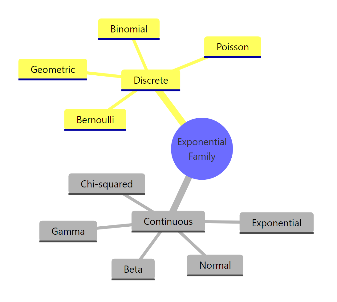
Common distributions that belong to the exponential family.

Figure 3: Common distributions that belong to the exponential family.

Key takeaways:

The canonical density factors data and parameter cleanly into $h(x) \exp\{\eta T(x) - A(\eta)\}$.
The sufficient statistic $T(x)$ is everything the data tell you about $\theta$, so MLE depends only on $T$ and $n$.
The natural-parameter map $\theta \to \eta$ is the GLM canonical link, identity for Normal, logit for Bernoulli, log for Poisson.
Differentiating the log-partition function once gives the mean of $T$, twice gives the variance.

References

Casella, G., & Berger, R. L. Statistical Inference, 2nd Edition. Duxbury (2002). Chapter 3.4: The exponential family. Link
Wikipedia. Exponential family. Link
DasGupta, A. The Exponential Family and Statistical Applications, Purdue University lecture notes. Link
Geyer, C. J. Stat 5421 Lecture Notes: Exponential Families, University of Minnesota. Link
Jordan, M. I. An Introduction to Probabilistic Graphical Models, Chapter 8: The exponential family. UC Berkeley. Link
R Core Team. The R Stats Package: glm(). Link
McCullagh, P., & Nelder, J. A. Generalized Linear Models, 2nd Edition. Chapman & Hall (1989). The original GLM textbook.

Continue Learning

Maximum Likelihood Estimation in R, how the score equation behind the canonical-link GLM works in detail.
Logistic Regression with R, the Bernoulli exponential family at work, with the logit link in front.
Poisson Regression in R, count-data modelling using the Poisson canonical form.