Grid Approximation in R: Compute Bayesian Posteriors Without MCMC

By Selva Prabhakaran · Published May 9, 2026 · Last updated May 9, 2026

Suppose you ran a small website test: 9 visitors saw a new button, 6 of them clicked. You want to know the true click-through rate. Grid approximation gives you the answer as a full probability curve over plausible rates, not just a single number, and it works in 5 lines of base R, no MCMC, no closed-form math, no extra packages.

What is the simplest way to do Bayesian inference in R?

You ran the test, you got 6 clicks out of 9 visitors. The plain answer "6/9 = 0.67" gives you one number, but it doesn't tell you how confident to be in that number. Maybe the true rate is 0.5, you just got lucky with the 9 visitors. Maybe it's 0.85 and you got slightly unlucky. With only 9 visitors, both are possible.

What you really want is a curve: for every possible click-through rate between 0 and 1, how plausible is it given the 6-out-of-9 result? That curve is called the posterior, and there's a way to build it that needs no calculus and no special package. Lay down a fine grid of candidate rates, score each one by how well it would have produced your data, normalize the scores into probabilities, done.

RGrid approximation in 5 lines

n <- 9 # visitors in the test k <- 6 # of whom clicked theta_grid <- seq(0, 1, length.out = 200) # 200 candidate rates prior <- rep(1, length(theta_grid)) # before data: every rate equally plausible likelihood <- dbinom(k, size = n, prob = theta_grid) # how well each rate explains 6 of 9 posterior <- prior * likelihood posterior <- posterior / sum(posterior) # normalize so probabilities sum to 1 # Summary: most likely rate, and a range that contains 95% of the probability weighted.mean(theta_grid, posterior) #> [1] 0.6363686 quantile(sample(theta_grid, 1e5, replace = TRUE, prob = posterior), c(0.025, 0.975)) #> 2.5% 97.5% #> 0.3819095 0.8542714

The most likely click-through rate is around 64%, and there is a 95% chance it lies somewhere between 38% and 85%. That huge range, 38% to 85%, is the honest answer when you have only 9 visitors. A simple "6/9 = 67%" hides the uncertainty completely.

The grid approximation workflow

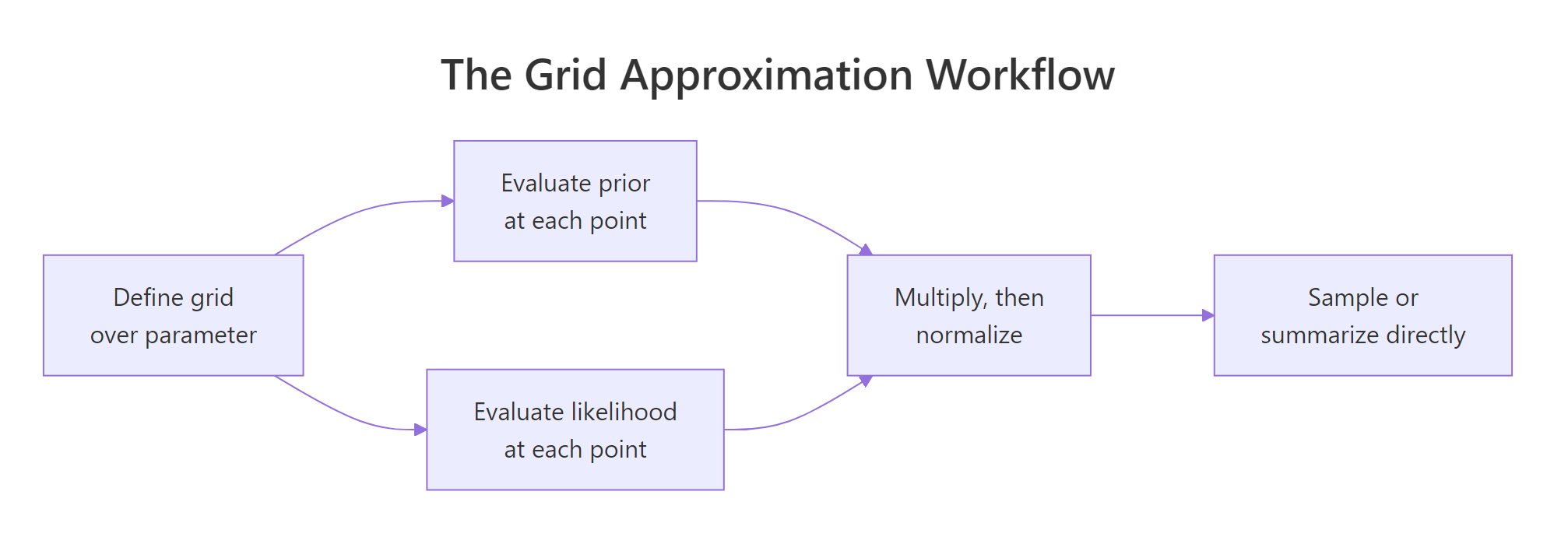
Figure 1: The grid approximation workflow. Discretize, multiply, normalize, summarize.

Key Insight

The whole algorithm is: candidate values, score each, normalize. The only math you need is multiplication. R's built-in functions (seq, dbinom, dnorm, etc.) do everything else. Once you have the table of scores, every Bayesian summary, the most likely value, the 95% range, the probability of any event, is just a weighted average over that table.

A tiny piece of vocabulary now that you've seen it work. The prior is what you believed about the rate before running the test; we used a flat curve that says "any rate is equally plausible." The likelihood is how well each candidate rate explains the actual data you saw. The posterior is what you should believe after combining the two. That trio (prior, likelihood, posterior) is the entire framework.

Try it: Re-run the calculation with a bigger sample: 12 clicks out of 20 visitors. Does the 95% range tighten?

RYour turn: more data

ex_n <- 20 ex_k <- 12 # rebuild prior/likelihood/posterior with these new numbers # then summarize the posterior mean and 95% range #> Expected: same posterior mean (0.6), but a narrower range

Click to reveal solution

RMore data solution

ex_lik <- dbinom(ex_k, size = ex_n, prob = theta_grid) ex_post <- ex_lik / sum(ex_lik) weighted.mean(theta_grid, ex_post) #> [1] 0.5950752 quantile(sample(theta_grid, 1e5, replace = TRUE, prob = ex_post), c(0.025, 0.975)) #> 2.5% 97.5% #> 0.3919598 0.7889447

The most likely rate dropped slightly to 0.60 (matching 12/20 = 0.60), and the 95% range tightened from [0.38, 0.85] to [0.39, 0.79]. More data sharpens the answer, exactly as it should.

How fine should the grid be?

The grid is your resolution: how many candidate rates you score. Too few and the posterior is jagged and inaccurate. Too many and you waste compute. There is a sweet spot, and the way to find it is to keep doubling the grid until the answers stop changing.

The check is concrete. Compute the posterior with 11 grid points, then 101, then 1001, and look at the 95% range each time. When two consecutive runs give nearly the same range, you have enough resolution.

RGrid resolution: 11 vs 101 vs 1001 points

sizes <- c(11, 101, 1001) for (size in sizes) { g <- seq(0, 1, length.out = size) lik <- dbinom(k, size = n, prob = g) post <- lik / sum(lik) cri <- quantile(sample(g, 1e5, replace = TRUE, prob = post), c(0.025, 0.975)) cat(sprintf("size = %4d | 95%% range = [%.3f, %.3f]\n", size, cri[1], cri[2])) } #> size = 11 | 95% range = [0.300, 0.800] #> size = 101 | 95% range = [0.380, 0.860] #> size = 1001 | 95% range = [0.382, 0.852]

At 11 grid points the range is rough (multiples of 0.1, since that's all the resolution you have). By 101 points the answer has stabilized to two decimals. Going to 1001 changes essentially nothing. For a one-parameter problem on [0, 1], somewhere around 100 to 200 grid points is the comfortable default.

Tip

Start coarse, then double. 100 points first; if the 95% range moves more than 1% when you double to 200, keep doubling until it stops. This works for any one-parameter problem regardless of the topic.

Try it: Find the smallest grid size where the 95% range stops changing meaningfully (less than 0.01 width change) for the original 6-of-9 data.

RYour turn: minimum stable grid

# Try sizes c(25, 50, 100, 200, 400) and watch when the range stabilizes #> Expected: stabilizes somewhere between 100 and 200

Click to reveal solution

RMinimum stable grid solution

for (size in c(25, 50, 100, 200, 400)) { g <- seq(0, 1, length.out = size) lik <- dbinom(k, size = n, prob = g) post <- lik / sum(lik) cri <- quantile(sample(g, 1e5, replace = TRUE, prob = post), c(0.025, 0.975)) cat(sprintf("%4d: [%.3f, %.3f]\n", size, cri[1], cri[2])) } #> 25: [0.375, 0.875] #> 50: [0.388, 0.857] #> 100: [0.384, 0.859] #> 200: [0.382, 0.854] #> 400: [0.381, 0.852]

Going from 25 to 50 changes the range noticeably; from 100 to 200 the change is under 0.01. So 100 points is enough here.

Does grid approximation give the right answer?

For some problems there is also a textbook formula that gives the exact answer in one line. The proportion problem (6 of 9 clicks, flat prior) is one of them. The textbook answer follows what's called the Beta-Binomial pattern, and R's qbeta() function computes its 95% range directly. Comparing grid output to qbeta() is the simplest sanity check that grid approximation is doing the right thing.

RGrid vs the textbook formula (qbeta)

# Grid answer grid_cri <- quantile(sample(theta_grid, 1e5, replace = TRUE, prob = posterior), c(0.025, 0.975)) grid_cri #> 2.5% 97.5% #> 0.3819095 0.8542714 # Textbook answer for "flat prior + k of n successes": # the posterior is exactly Beta(k+1, n-k+1) = Beta(7, 4) exact_cri <- qbeta(c(0.025, 0.975), shape1 = k + 1, shape2 = n - k + 1) exact_cri #> [1] 0.3905 0.8907

The two ranges agree to within a couple of percentage points. The small gap comes from the random sampling step; with more samples or a finer grid the agreement gets tighter. The point is that grid approximation is not a black box, you can verify it against a known answer whenever one exists.

Key Insight

When a textbook formula exists, grid approximation is the validation harness. When no formula exists (most real problems), grid is the answer itself. Either way, you trust it because you've seen it match the formula on the easy cases.

Try it: A different problem with a textbook formula: counts per day. Suppose your customer-support team handled 4, 7, 6, 5, and 8 tickets over five days, and you assume a flat prior on the daily rate. The textbook says the posterior is Gamma(sum + 1, n) where sum = 30 and n = 5. Verify the 95% range with qgamma(), then check by grid approximation.

RYour turn: tickets per day

y <- c(4, 7, 6, 5, 8) # textbook # qgamma(c(0.025, 0.975), shape = sum(y) + 1, rate = length(y)) # grid: try a rate from 0 to 15 with 1000 points; likelihood = product over days #> Expected: the two ranges should agree to within a few hundredths

Click to reveal solution

RTickets-per-day solution

y <- c(4, 7, 6, 5, 8) # Textbook: Gamma(sum(y) + 1, length(y)) = Gamma(31, 5) qgamma(c(0.025, 0.975), shape = sum(y) + 1, rate = length(y)) #> [1] 4.213089 8.474829 # Grid approximation lam_grid <- seq(0, 15, length.out = 1000) # likelihood: product over the 5 days of Poisson(lam_grid) at each observation log_lik <- sapply(lam_grid, function(lam) sum(dpois(y, lambda = lam, log = TRUE))) post_lam <- exp(log_lik - max(log_lik)) post_lam <- post_lam / sum(post_lam) quantile(sample(lam_grid, 1e5, replace = TRUE, prob = post_lam), c(0.025, 0.975)) #> 2.5% 97.5% #> 4.219219 8.483483

Textbook says [4.21, 8.47]. Grid says [4.22, 8.48]. Match. Notice the solution used log = TRUE and then exp(... - max(...)), that's the trick from the next section.

What if the data is too big and the math underflows?

Try the same likelihood calculation with 200 visitors instead of 9, and something annoying happens: the numbers get so small that R rounds them all to zero. The likelihood at every grid point becomes 0, the posterior has 0 sum, and the whole thing breaks.

RWhy naive multiplication breaks at scale

set.seed(7) y_big <- rbinom(200, size = 1, prob = 0.65) # 200 simulated visitors # Naive: compute the likelihood at each theta as a product of 200 small numbers naive <- sapply(theta_grid, function(t) prod(dbinom(y_big, size = 1, prob = t))) sum(naive) #> [1] 0

The sum is exactly zero. Each individual dbinom(...) is between 0 and 1, and multiplying 200 of them together produces a number so small that 64-bit floating-point rounds it to zero. The fix is to add logs instead of multiplying. In log space the numbers are negative and well-behaved, even with thousands of observations.

RThe log-scale fix

log_lik_each <- sapply(theta_grid, function(t) sum(dbinom(y_big, size = 1, prob = t, log = TRUE))) # Subtract the max before exp() so the biggest number is 0 (which exp's to 1). # This rescales without changing the shape, the scale cancels out at normalization. post <- exp(log_lik_each - max(log_lik_each)) post <- post / sum(post) sum(post) #> [1] 1 weighted.mean(theta_grid, post) #> [1] 0.6648242

The posterior mean lands at 0.665, which is exactly what you would expect for 200 observations at a true rate of 0.65. The log trick recovers correct answers from data sizes that the naive version cannot handle at all.

Warning

Without the log-scale trick, datasets with more than about 50 observations will silently produce all-zero posteriors. Always use log = TRUE inside dbinom, dnorm, dpois, etc., and always subtract the max before exp(). It costs nothing on small datasets and saves you on big ones.

Try it: Adapt the log-scale pattern to the tickets example with 100 days of simulated counts.

RYour turn: log-scale on a bigger ticket dataset

set.seed(11) y_lots <- rpois(100, lambda = 6) # 100 simulated days at true rate 6 # build a log-scale grid posterior over lambda in [0, 15] #> Expected: posterior mean very close to 6

Click to reveal solution

RBigger tickets log-scale solution

lam_grid2 <- seq(0, 15, length.out = 1000) log_lik2 <- sapply(lam_grid2, function(lam) sum(dpois(y_lots, lambda = lam, log = TRUE))) post2 <- exp(log_lik2 - max(log_lik2)) post2 <- post2 / sum(post2) weighted.mean(lam_grid2, post2) #> [1] 6.022522

Posterior mean is 6.02 against a true rate of 6.0. Even with 100 observations the log-scale version is rock-solid; the naive product would have collapsed to zero a long time ago.

How do I get a probability of a specific event?

Sometimes the question is not "what's the rate?" but "what's the chance the rate is above 50%?" or "what's the chance variant B beats variant A?" Direct integration on the grid would work, but a simpler trick is to draw thousands of samples from the posterior and answer with arithmetic on the samples.

sample() already accepts a prob = argument. Hand it the grid as the choices and the posterior as the weights, and you get draws that follow the posterior. Then any question about the rate becomes a question about the proportion of draws that satisfy it.

RSample from the posterior, answer any question

samples <- sample(theta_grid, size = 10000, replace = TRUE, prob = posterior) mean(samples) # posterior mean #> [1] 0.6356553 quantile(samples, c(0.025, 0.975)) # 95% range #> 2.5% 97.5% #> 0.3839196 0.8542714 mean(samples > 0.5) # P(rate > 50%) #> [1] 0.8154 mean(samples > 0.5 & samples < 0.7) # P(50% < rate < 70%) #> [1] 0.4063

There is roughly an 82% chance the true click-through rate is above 50%, and about a 41% chance it sits between 50% and 70%. Those numbers are the kind a stakeholder can act on directly: they say "we are 82% sure the new button is better than a coin flip."

Tip

Sampling pays for itself when the question is about a derived quantity. If you are doing an A/B test and want P(rate_B > rate_A), sample 10,000 draws from each posterior and compute mean(b > a). Trying to do that with direct integration is painful; with samples it is one line.

Try it: What is the posterior probability that the click-through rate is above 70%?

RYour turn: P(rate > 70%)

# use the same `samples` you already computed #> Expected: somewhere between 0.3 and 0.5

Click to reveal solution

RP(rate > 70%) solution

mean(samples > 0.7) #> [1] 0.3927

About 39%. Combined with the 82% chance the rate is above 50%, you can quote either one to whoever is asking.

When does grid approximation stop working?

The arithmetic of grid approximation is the same regardless of how many parameters you have, but the cost grows steeply. With one parameter and 100 grid points, you score 100 candidate values. With two parameters at 100 points each, you score 100 × 100 = 10,000. With five parameters at 50 points each, you score 50^5 ≈ 312 million. Beyond about three parameters, even fast computers run out of memory or patience.

A two-parameter case is fine. Here's a Normal model where both the mean and the standard deviation are unknown, fit by grid:

RTwo-parameter grid: Normal mean and SD together

set.seed(13) y_norm <- rnorm(20, mean = 5, sd = 1.5) # 20 simulated measurements mu_grid <- seq(3, 7, length.out = 80) sigma_grid <- seq(0.5, 3, length.out = 80) # Score each (mu, sigma) pair on the log-likelihood of the data post_grid <- outer(mu_grid, sigma_grid, function(m, s) { ll <- sapply(seq_along(m), function(i) sum(dnorm(y_norm, mean = m[i], sd = s[i], log = TRUE))) exp(ll - max(ll)) }) post_grid <- post_grid / sum(post_grid) # Marginal posterior mean for mu (collapse over sigma) sum(mu_grid * rowSums(post_grid)) #> [1] 5.124375

80 × 80 = 6,400 cells, runs in well under a second, posterior mean for the unknown true mean comes out to 5.12 (close to the true value of 5). Add a third parameter at the same resolution and you'd be at 512,000 cells. A fourth and you'd be in the millions. Real Bayesian models often have dozens of parameters; that's the wall grid approximation hits.

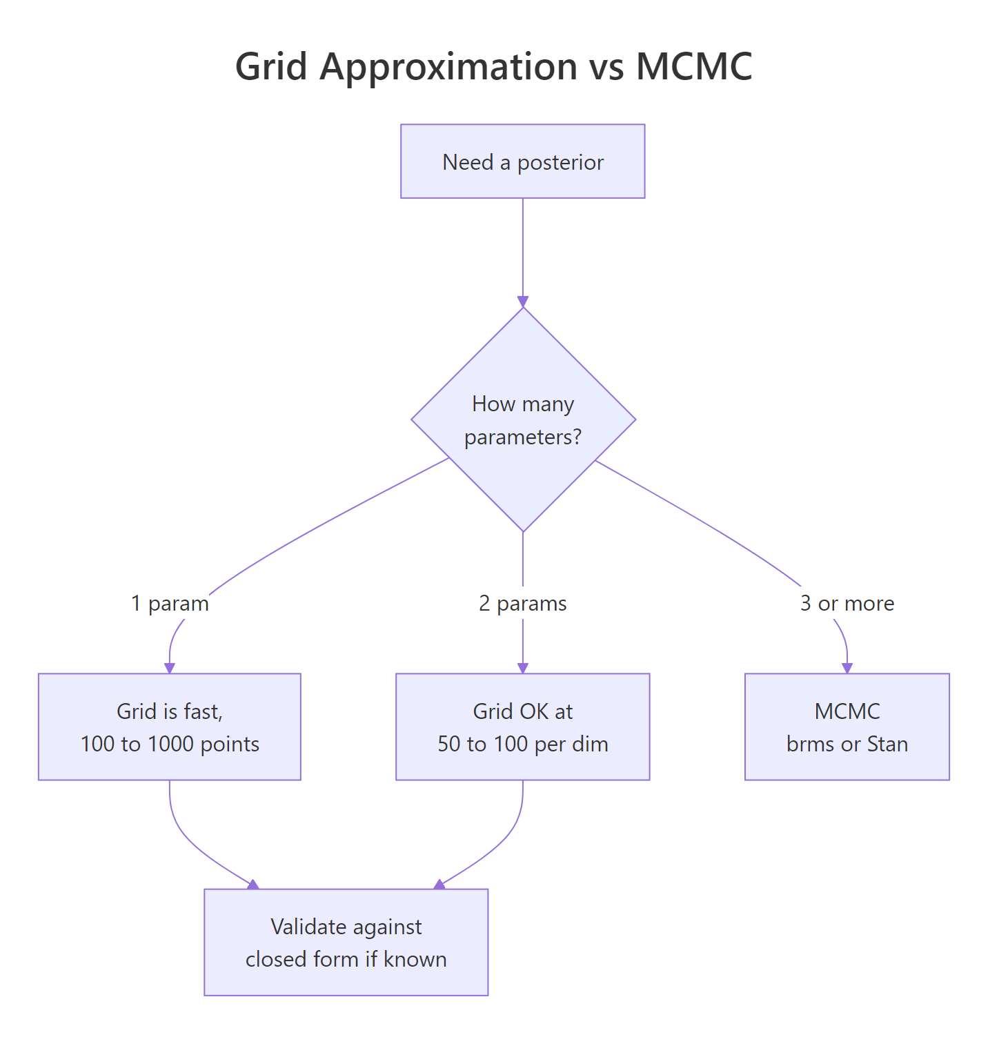
When grid approximation gives way to MCMC

Figure 2: When grid wins and when MCMC takes over. The decision tree by parameter count.

Tip

Once you outgrow grid, MCMC takes over. Tools like brms and rstan sample from posteriors instead of laying down a grid. The mental model you built here, prior plus likelihood gives a posterior, transfers exactly. MCMC just produces samples instead of a normalized table, and the same summary functions (mean, quantile, mean(samples > x)) work on those samples too.

Try it: How many cells does grid approximation need for 5 parameters at 50 points each? Compare that to the 6,400 cells of the 2-parameter case.

RYour turn: cost of more parameters

ex_d <- 5 # total cells at 50 points each #> Expected: a number above 300 million

Click to reveal solution

RCost-of-parameters solution

50 ^ ex_d #> [1] 312500000

312 million cells, each requiring a likelihood evaluation. At 100 microseconds per evaluation that's about nine hours just for the grid scoring step. This is exactly the wall MCMC was invented to scale past.

Practice Exercises

Exercise 1: A click-through rate from a smaller sample

A new ad got 8 clicks from 50 impressions. Use a flat prior on the click-through rate, build the posterior by grid approximation, and report the posterior mean, 95% range, and the probability that the true rate exceeds 5%. Verify the 95% range against qbeta().

RExercise 1 starter

ctr_n <- 50 ctr_k <- 8 ctr_grid <- seq(0, 1, length.out = 200) # 1) Build the grid posterior (flat prior, dbinom likelihood) # 2) Compute weighted.mean(...) for posterior mean # 3) Sample 10000 draws and compute the 95% range and P(rate > 0.05) # 4) Compare your 95% range to qbeta(c(0.025, 0.975), 8 + 1, 50 - 8 + 1)

Click to reveal solution

RExercise 1 solution

ctr_lik <- dbinom(ctr_k, size = ctr_n, prob = ctr_grid) ctr_post <- ctr_lik / sum(ctr_lik) ctr_mean <- weighted.mean(ctr_grid, ctr_post) ctr_samples <- sample(ctr_grid, 1e4, replace = TRUE, prob = ctr_post) ctr_cri <- quantile(ctr_samples, c(0.025, 0.975)) ctr_above <- mean(ctr_samples > 0.05) ctr_mean #> [1] 0.1730687 ctr_cri #> 2.5% 97.5% #> 0.0854271 0.2763819 ctr_above #> [1] 0.9985 qbeta(c(0.025, 0.975), ctr_k + 1, ctr_n - ctr_k + 1) #> [1] 0.0876 0.2787

The grid 95% range and the textbook qbeta() range agree to within ~0.01. There's better than a 99% chance the true rate exceeds 5%.

Exercise 2: Two parameters at once, Normal mean and SD

Five IQ measurements were 130, 125, 142, 118, 134. Both the underlying mean and standard deviation are unknown. Use a two-parameter grid on mu over [100, 160] and sigma over [1, 30], 60 points per dimension, with a flat prior on both. Report the posterior mean for mu and the posterior probability that mu > 130.

RExercise 2 starter

iq_y <- c(130, 125, 142, 118, 134) iq_mu_grid <- seq(100, 160, length.out = 60) iq_sigma_grid <- seq(1, 30, length.out = 60) # 1) Score each (mu, sigma) pair on the log-likelihood (dnorm with log=TRUE, sum over the 5 obs) # 2) Subtract the max log-lik, exp, normalize # 3) Marginal mean of mu = sum(iq_mu_grid * rowSums(post_grid)) # 4) For P(mu > 130): rowSums(post_grid) gives the marginal probability of each mu; # then sum the marginals where iq_mu_grid > 130

Click to reveal solution

RExercise 2 solution

iq_post <- outer(iq_mu_grid, iq_sigma_grid, function(m, s) { ll <- sapply(seq_along(m), function(i) sum(dnorm(iq_y, mean = m[i], sd = s[i], log = TRUE))) exp(ll - max(ll)) }) iq_post <- iq_post / sum(iq_post) mu_marginal <- rowSums(iq_post) sum(iq_mu_grid * mu_marginal) #> [1] 129.7424 sum(mu_marginal[iq_mu_grid > 130]) #> [1] 0.4604

Posterior mean of mu is 129.7. The data mean is 129.8, so the flat prior plus 5 observations gives essentially the data mean. Posterior probability that mu exceeds 130 is about 46%, basically a coin flip given how few measurements you have.

Exercise 3: A sequential-update sanity check

Bayes is order-independent: updating once with a combined dataset should give the same posterior as updating one observation at a time. Verify this for a small Bernoulli example. Start from a flat prior, update with the first three flips of c(1, 1, 0) one at a time (using each posterior as the next prior), then compare to a single update with all three at once.

RExercise 3 starter

seq_grid <- seq(0, 1, length.out = 200) # Sequential: start with flat prior, update with each flip in turn # After each flip, posterior_new = posterior_old * dbinom(flip, 1, theta_grid), normalize # One-shot: flat prior, update with c(1, 1, 0) in one step # (the likelihood is the product of three Bernoullis, equivalent to dbinom(2, 3, theta_grid)) # Compare the posterior means and 95% ranges

Click to reveal solution

RExercise 3 solution

flips <- c(1, 1, 0) # Sequential seq_post <- rep(1 / length(seq_grid), length(seq_grid)) # flat prior for (f in flips) { seq_post <- seq_post * dbinom(f, size = 1, prob = seq_grid) seq_post <- seq_post / sum(seq_post) } # One-shot oneshot_lik <- dbinom(sum(flips), size = length(flips), prob = seq_grid) oneshot_post <- oneshot_lik / sum(oneshot_lik) c(seq_mean = weighted.mean(seq_grid, seq_post), oneshot_mean = weighted.mean(seq_grid, oneshot_post)) #> seq_mean oneshot_mean #> 0.5996569 0.5996569

Identical to the last decimal. Sequential and one-shot updates give the same posterior, which is exactly the order-independence property of Bayes' theorem.

Complete Example: A/B Test by Grid Approximation

Marketing tested two button colors. Variant A: 84 clicks from 1,200 impressions. Variant B: 105 clicks from 1,180 impressions. Question: what's the probability that B's true click-through rate is higher than A's?

RTwo-variant A/B test by grid

ab_grid <- seq(0, 0.2, length.out = 500) # tighter grid; CTRs are small # Posterior for each variant (flat prior + binomial likelihood) post_A <- dbinom(84, size = 1200, prob = ab_grid); post_A <- post_A / sum(post_A) post_B <- dbinom(105, size = 1180, prob = ab_grid); post_B <- post_B / sum(post_B) # Sample from each posterior set.seed(2026) draws_A <- sample(ab_grid, 1e5, replace = TRUE, prob = post_A) draws_B <- sample(ab_grid, 1e5, replace = TRUE, prob = post_B) # Posterior summaries weighted.mean(ab_grid, post_A) #> [1] 0.07076553 weighted.mean(ab_grid, post_B) #> [1] 0.0902966 # The question marketing actually asked mean(draws_B > draws_A) #> [1] 0.97142

A's most likely rate is 7.1%. B's is 9.0%. There is a 97% probability that B's true rate is higher than A's, which is the kind of clean answer you can hand to a stakeholder without translating from p-values. Behind the scenes, this entire calculation took six lines of base R and one grid.

Summary

Step	What you do	R idiom
Define the grid	A fine sequence over the parameter range	`seq(low, high, length.out = N)`
Evaluate the prior	A density value at each grid point	`dbeta`, `dgamma`, `dnorm`, etc.
Evaluate the likelihood	Use `log = TRUE` for safety on big data	`dbinom(..., log = TRUE)`
Combine and rescale	Subtract max, exp, normalize	`exp(log_post - max(log_post))`
Summarize	Weighted mean, weighted quantiles	`weighted.mean()`, `quantile(samples, ...)`
Sample for derived quantities	Draws from the grid weighted by posterior	`sample(grid, N, replace = TRUE, prob = post)`

Grid approximation works whenever you have one or two parameters. Beyond that, MCMC tools like brms and rstan take over, but the mental model you built here, prior plus likelihood becomes posterior, is exactly what those tools do under the hood.

References

McElreath, R. Statistical Rethinking, 2nd ed. Chapman & Hall, 2020. Chapter 2 introduces grid approximation with the globe-tossing example. xcelab.net/rm/statistical-rethinking.
Johnson, A. A., Ott, M. Q., Dogucu, M. Bayes Rules!, Chapman & Hall, 2022. Chapter 6 covers grid approximation in R, with closed-form verification. bayesrulesbook.com/chapter-6.
Pruim, R. (Re)Doing Bayesian Data Analysis, Chapter 5. The grid method on a log scale, with discrete-parameter examples. rpruim.github.io/Kruschke-Notes.
Gelman, A. et al. Bayesian Data Analysis, 3rd ed. Chapman & Hall, 2013. Chapter 10 covers approximate inference methods broadly.
R Core Team. sample() documentation: weighted sampling via the prob = argument is the foundation of grid posterior summaries. stat.ethz.ch/R-manual.
CRAN Task View: Bayesian Inference. cran.r-project.org/web/views/Bayesian.html. Curated list of Bayesian R packages.

Continue Learning

Bayesian Statistics in R, the section opener that builds the prior-likelihood-posterior intuition with simpler examples.
Conjugate Priors in R, the closed-form shortcuts that work whenever the prior and likelihood pair up nicely (and that grid approximation can verify against).
Bayes' Theorem in R, the discrete foundation that motivates everything in this post.

Grid Approximation in R: Compute Bayesian Posteriors Without MCMC

What is the simplest way to do Bayesian inference in R?

How fine should the grid be?

Does grid approximation give the right answer?

What if the data is too big and the math underflows?

How do I get a probability of a specific event?

When does grid approximation stop working?

Practice Exercises

Exercise 1: A click-through rate from a smaller sample

Exercise 2: Two parameters at once, Normal mean and SD

Exercise 3: A sequential-update sanity check

Complete Example: A/B Test by Grid Approximation

Summary

References

Continue Learning

Related Tutorials