Mann-Whitney U Test in R: Two Independent Groups, Distribution-Free

The Mann-Whitney U test compares two independent groups when the data are not normal or are ordinal. In R, wilcox.test(y ~ group) returns the U statistic and a p-value without assuming any distribution.

How do you run a Mann-Whitney U test in R?

Suppose you want to know whether automatic and manual cars get different miles per gallon, but a few outliers are pulling the means around. The Mann-Whitney U test ranks every observation across both groups and compares the rank totals, so a single odd value cannot dominate the result. One call to wilcox.test() does the whole thing.

RRun wilcox.test on mtcars mpg by transmission

# Split mpg by transmission: am = 0 is automatic, am = 1 is manual mpg_auto <- mtcars$mpg[mtcars$am == 0] mpg_manual <- mtcars$mpg[mtcars$am == 1] mw_result <- wilcox.test(mpg_auto, mpg_manual) mw_result #> #> Wilcoxon rank sum test with continuity correction #> #> data: mpg_auto and mpg_manual #> W = 42, p-value = 0.001871 #> alternative hypothesis: true location shift is not equal to 0

The U statistic (R prints it as W) is 42, and the p-value is 0.001871. With p well below 0.05, you reject the null that automatic and manual cars come from the same distribution: manual cars get systematically more miles per gallon. That is your answer in three lines of code, no normality assumed.

Note

R calls the test "Wilcoxon rank sum" but it is the same as Mann-Whitney U. Mann and Whitney later showed their U is a simple linear function of Wilcoxon's W, so the two names refer to one test. R uses Wilcoxon's label, but the p-value is identical.

Try it: Use wilcox.test() to compare Sepal.Length between the setosa and versicolor species in the iris dataset. Save the result to ex_iris_mw and print it.

RYour turn: Mann-Whitney on iris Sepal.Length

# Subset Sepal.Length for setosa and versicolor ex_setosa <- iris$Sepal.Length[iris$Species == "setosa"] ex_versicolor <- iris$Sepal.Length[iris$Species == "versicolor"] ex_iris_mw <- # your code here ex_iris_mw #> Expected: a Wilcoxon rank sum test result with W and a very small p-value

Click to reveal solution

RIris setosa vs versicolor solution

ex_setosa <- iris$Sepal.Length[iris$Species == "setosa"] ex_versicolor <- iris$Sepal.Length[iris$Species == "versicolor"] ex_iris_mw <- wilcox.test(ex_setosa, ex_versicolor) ex_iris_mw #> Wilcoxon rank sum test with continuity correction #> data: ex_setosa and ex_versicolor #> W = 168.5, p-value = 8.346e-14

Explanation: Setosa flowers have far shorter sepals than versicolor, so the rank sums diverge and the p-value is essentially zero.

When should you use Mann-Whitney over a t-test?

The two-sample t-test asks whether two group means differ, and it trusts the Central Limit Theorem to keep the math honest. That trust falls apart with skewed data, ordinal scales, or small samples with outliers. The Mann-Whitney U test side-steps the problem by working on ranks, which compress big values and pull in the tails.

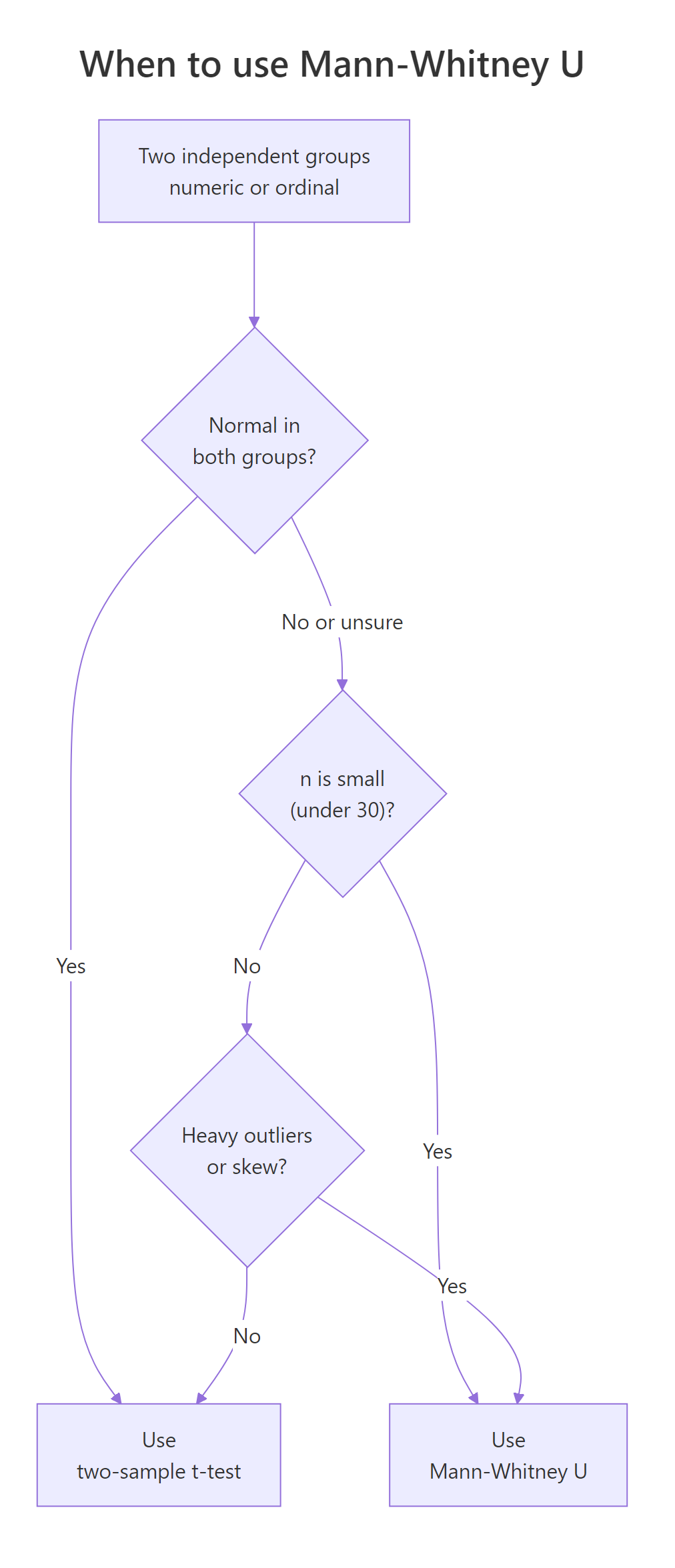
When to choose Mann-Whitney U over a two-sample t-test.

Figure 1: When to choose Mann-Whitney U over a two-sample t-test.

Let's see what happens when the t-test's normality assumption is wrong. We will simulate two heavily right-skewed samples and run both tests on the same data.

RCompare t-test and Mann-Whitney on skewed data

set.seed(73) skewed_a <- rexp(20, rate = 1.0) # mean ~1.0 skewed_b <- rexp(20, rate = 0.7) # mean ~1.43 t_p <- t.test(skewed_a, skewed_b)$p.value mw_p <- wilcox.test(skewed_a, skewed_b)$p.value c(t_test = round(t_p, 4), mann_whitney = round(mw_p, 4)) #> t_test mann_whitney #> 0.1010 0.0479

Same data, two different verdicts. The t-test gives p = 0.1010 (not significant), while the Mann-Whitney returns p = 0.0479 (significant at 5%). The skew inflated the t-test's variance estimate and washed out the signal; ranks did not care.

Key Insight

Mann-Whitney does not test medians, it tests stochastic dominance. A significant p-value means values from one group tend to be larger than values from the other, not that the medians differ. The two are equivalent only when the two distributions have the same shape. Always look at the boxplots before you write "the medians differ."

Try it: You collect a 5-point Likert satisfaction score (1 = bad, 5 = great) from two product variants, n = 12 each. Which test fits the data, and why? Set your answer as a string in ex_choice.

RYour turn: pick the right test

# Likert data is ordinal, n is small, normality is unrealistic. ex_choice <- # your code here ex_choice #> Expected: "Mann-Whitney" with a one-line reason

Click to reveal solution

RLikert test choice solution

ex_choice <- "Mann-Whitney: Likert is ordinal, not interval, and n=12 is too small to lean on the CLT." ex_choice #> [1] "Mann-Whitney: Likert is ordinal, not interval, and n=12 is too small to lean on the CLT."

Explanation: Likert ratings have ranked spacing but unequal psychological distances between points, so a t-test on the raw integers misrepresents the data.

How do you run the test from a data frame using formulas?

Splitting a column into two vectors before testing is fine for two groups, but it gets tedious fast. R's formula syntax keeps the data frame intact and reads almost like a sentence: outcome ~ group. The result is identical to the vector form, but the code is cleaner and ports straight to other modelling functions.

The formula mpg ~ am says "model mpg by am." Inside wilcox.test(), that becomes "compare mpg between the two levels of am." The data = mtcars argument tells R where to find both columns.

RUse formula syntax with wilcox.test

mw_formula <- wilcox.test(mpg ~ am, data = mtcars) mw_formula #> #> Wilcoxon rank sum test with continuity correction #> #> data: mpg by am #> W = 42, p-value = 0.001871 #> alternative hypothesis: true location shift is not equal to 0

Same W = 42, same p = 0.001871. The formula form costs one line and gives you free integration with subset = filters and dplyr pipelines. Use it whenever your data already lives in a tidy data frame.

Tip

Use the formula form for inline filters. wilcox.test(mpg ~ am, data = mtcars, subset = cyl != 8) runs the test on 4- and 6-cylinder cars only, no preprocessing needed. The vector form would force a separate filter step.

Try it: Use the chickwts dataset (chicken weights by feed type). Run a Mann-Whitney U test comparing casein and horsebean feeds using formula syntax and store it in ex_chick_mw.

RYour turn: chickwts casein vs horsebean

ex_chick_mw <- # your code here ex_chick_mw #> Expected: a wilcox.test result comparing casein and horsebean weights

Click to reveal solution

RChickwts feed comparison solution

ex_chick_mw <- wilcox.test(weight ~ feed, data = chickwts, subset = feed %in% c("casein", "horsebean")) ex_chick_mw #> Wilcoxon rank sum test with continuity correction #> data: weight by feed #> W = 140, p-value = 1.235e-05

Explanation: subset = feed %in% c(...) keeps only the two levels you want. Casein-fed chicks weigh far more, so the p-value is tiny.

How do you visualize the two groups before testing?

A test gives you a number. A picture tells you what that number means. Before you trust any p-value, plot the two groups so you can see the shape, the spread, and any outliers. If the two distributions look wildly different in shape, the test still runs, but your interpretation must change.

We will use ggplot2 to draw a boxplot of mpg by am, with am cast as a factor so it reads as a category instead of a number.

RBoxplot of mpg by transmission

library(ggplot2) gg_box <- ggplot(mtcars, aes(x = factor(am, labels = c("Automatic", "Manual")), y = mpg)) + geom_boxplot(fill = "#a78bfa", alpha = 0.7) + labs(x = "Transmission", y = "Miles per gallon", title = "mtcars: mpg by transmission") + theme_minimal() gg_box #> A boxplot with manual cars centred well above automatic cars

The manual box sits clearly above the automatic box, and the spreads are roughly comparable. That visual is what makes the p = 0.001871 from earlier feel right rather than mysterious.

A density plot adds detail the boxplot hides, namely the shape of each group and any hint of bimodality.

RDensity plot of mpg by transmission

gg_density <- ggplot(mtcars, aes(x = mpg, fill = factor(am, labels = c("Automatic", "Manual")))) + geom_density(alpha = 0.5) + scale_fill_manual(values = c("#a78bfa", "#34d399"), name = "Transmission") + labs(x = "Miles per gallon", y = "Density", title = "Distribution of mpg by transmission") + theme_minimal() gg_density #> Two overlapping density curves; the manual curve is shifted right

Both curves are roughly symmetric, the manual curve is shifted right, and the shapes are similar. With matching shapes you can interpret the Mann-Whitney result as "manual cars have a higher median mpg." If the shapes had differed, you would phrase it more cautiously as "manual cars tend to have higher mpg."

Warning

Different distribution shapes change the conclusion you can draw. The test is valid either way, but only matched shapes let you talk about medians. Mismatched shapes force the looser language of stochastic dominance: "values in group A tend to be larger than values in group B."

Try it: Add a violin plot layer on top of the boxplot for mpg by am. Save the plot to ex_violin.

RYour turn: violin + boxplot

ex_violin <- ggplot(mtcars, aes(x = factor(am), y = mpg)) + # your code here theme_minimal() ex_violin #> Expected: violin shapes with boxplots overlaid inside them

Click to reveal solution

RViolin plus boxplot solution

ex_violin <- ggplot(mtcars, aes(x = factor(am, labels = c("Automatic", "Manual")), y = mpg)) + geom_violin(fill = "#a78bfa", alpha = 0.5) + geom_boxplot(width = 0.15, fill = "white") + labs(x = "Transmission", y = "Miles per gallon") + theme_minimal() ex_violin #> Violin shapes with thin white boxplots inside them

Explanation: geom_violin() shows the full density, and a narrow geom_boxplot() overlay keeps the median and quartiles visible.

How do you measure effect size for Mann-Whitney?

A p-value tells you whether a difference is real. An effect size tells you whether it is worth caring about. With large samples, even tiny differences become statistically significant; without an effect size, you cannot tell a meaningful gap from a trivial one.

How the U statistic is built from ranks across both groups.

Figure 2: How the U statistic is built from ranks across both groups.

The natural effect size for the Mann-Whitney test is the rank-biserial correlation, which Kerby (2014) showed equals the simple difference between the proportion of pair comparisons where group A wins and the proportion where group B wins. The Wendt formula computes it directly from the U statistic and the two group sizes.

$$r_{rb} = 1 - \frac{2U}{n_1 \cdot n_2}$$

Where:

$U$ = the W statistic R prints from wilcox.test()
$n_1$ = size of the first group passed to the test
$n_2$ = size of the second group

RCompute rank-biserial r from U

n1 <- length(mpg_auto) n2 <- length(mpg_manual) U_stat <- mw_result$statistic # this is W from wilcox.test r_rb <- 1 - (2 * U_stat) / (n1 * n2) unname(round(r_rb, 3)) #> [1] 0.66

The rank-biserial correlation is 0.66. The sign tells you the direction: a positive value means group 2 (manual) tends to have larger values, since R orders levels alphabetically (or by factor levels) when it computes U. The magnitude tells you the strength.

RInterpret effect size magnitude

effect_size <- abs(r_rb) interpretation <- dplyr::case_when( effect_size < 0.10 ~ "negligible", effect_size < 0.30 ~ "small", effect_size < 0.50 ~ "medium", TRUE ~ "large" ) unname(interpretation) #> [1] "large"

Cohen's thresholds for r rate 0.66 as a large effect, which lines up with the visual gap in the boxplot. Always report the effect size with three decimals plus a verbal label so the reader does not need to remember the cutoffs.

Tip

Pair every Mann-Whitney p-value with rank-biserial r and a 95% confidence interval for the location shift. The p-value answers "is there a difference?", the effect size answers "how big?", and the CI answers "what range is plausible?". Reviewers expect all three.

Try it: Compute the rank-biserial correlation for the setosa vs versicolor Sepal.Length test from the first exercise. Use ex_iris_mw$statistic. Save it to ex_iris_r.

RYour turn: rank-biserial r for iris

ex_n1 <- length(ex_setosa) ex_n2 <- length(ex_versicolor) ex_iris_r <- # your code here round(unname(ex_iris_r), 3) #> Expected: a value close to -1, signalling a very large effect

Click to reveal solution

RIris rank-biserial solution

ex_n1 <- length(ex_setosa) ex_n2 <- length(ex_versicolor) ex_iris_r <- 1 - (2 * ex_iris_mw$statistic) / (ex_n1 * ex_n2) round(unname(ex_iris_r), 3) #> [1] -0.866

Explanation: The negative sign means setosa values rank below versicolor values. The magnitude 0.866 is a very large effect.

How do you handle ties, small samples, and one-sided tests?

Three real-world wrinkles trip up beginners: tied values, small samples, and one-sided hypotheses. Each has a one-line fix.

When two or more observations share the same value, R cannot compute the exact p-value and prints a warning. The fix is to switch to the asymptotic approximation with exact = FALSE. The continuity correction stays on by default and adjusts for the discrete-to-continuous jump.

RHandle ties with exact = FALSE

# Two small samples with intentional ties tied_data_a <- c(2, 4, 4, 6, 7, 9) tied_data_b <- c(3, 4, 5, 7, 8, 8) mw_tied <- wilcox.test(tied_data_a, tied_data_b, exact = FALSE) mw_tied #> #> Wilcoxon rank sum test with continuity correction #> #> data: tied_data_a and tied_data_b #> W = 15.5, p-value = 0.6991 #> alternative hypothesis: true location shift is not equal to 0

No warning, and the p-value (0.6991) is reliable for any sample where ties are common. The half-rank in W = 15.5 shows that R averaged the ranks for the tied 4s and 7s.

Note

Use exact = TRUE only when n is small AND there are no ties. Default exact = NULL lets R decide based on sample size and ties. Forcing exact = TRUE with ties produces the warning and falls back to the same approximation anyway.

For a directional question, like "is automatic mpg lower than manual mpg?", swap the two-sided default for a one-sided test. The argument names are intuitive once you read them as "the first group's location is less/greater than the second's."

ROne-sided test with confidence interval

mw_one_sided <- wilcox.test(mpg_auto, mpg_manual, alternative = "less", conf.int = TRUE) mw_one_sided #> #> Wilcoxon rank sum test with continuity correction #> #> data: mpg_auto and mpg_manual #> W = 42, p-value = 0.0009356 #> alternative hypothesis: true location shift is less than 0 #> 95 percent confidence interval: #> -Inf -3.499975 #> sample estimates: #> difference in location #> -5.700017

The one-sided p-value (0.0009) is exactly half the two-sided value when the test agrees with the direction. The 95% CI for the location shift, $(-\infty, -3.5)$, says manual cars get at least 3.5 mpg more than automatics with 95% confidence.

Try it: Run a one-sided test on mtcars checking whether mpg_auto is less than mpg_manual, but this time on the data frame using formula syntax. Save it to ex_one_sided.

RYour turn: one-sided formula test

ex_one_sided <- # your code here ex_one_sided$p.value #> Expected: a small p-value matching the directional hypothesis

Click to reveal solution

ROne-sided formula solution

ex_one_sided <- wilcox.test(mpg ~ am, data = mtcars, alternative = "less") ex_one_sided$p.value #> [1] 0.0009356218

Explanation: With formula notation, alternative = "less" means level 0 (automatic) has a lower location than level 1 (manual). The p-value matches the vector form to the last digit.

How do you report Mann-Whitney U test results?

A solid report sentence packs the test name, group sizes, statistic, p-value, effect size, and effect direction into one line. Reviewers and readers can verify everything they need without rerunning your code.

The template below uses paste0() so it works in vanilla base R. Plug in your numbers and you have a publication-ready sentence.

RBuild a publication-ready report sentence

report <- paste0( "A Mann-Whitney U test showed that manual cars (n = ", n2, ") had higher mpg than automatic cars (n = ", n1, "), W = ", U_stat, ", p = ", signif(mw_result$p.value, 3), ", rank-biserial r = ", round(unname(r_rb), 2), "." ) cat(report) #> A Mann-Whitney U test showed that manual cars (n = 13) had higher mpg than automatic cars (n = 19), W = 42, p = 0.00187, rank-biserial r = 0.66.

That is one sentence, six numbers, zero ambiguity. Drop it straight into a results paragraph.

Tip

Always include n per group, U, p, effect size, and a 95% CI in the report. Without n the reader cannot judge power; without effect size they cannot judge importance; without CI they cannot judge precision. Strip any of those and a careful reviewer will ask for it.

Try it: Build a similar one-line report for the iris setosa-vs-versicolor result. Save the string to ex_iris_report.

RYour turn: format the iris result

ex_iris_report <- # your code here cat(ex_iris_report) #> Expected: a sentence with n per group, W, p, and rank-biserial r

Click to reveal solution

RIris report solution

ex_iris_report <- paste0( "A Mann-Whitney U test showed setosa (n = ", ex_n1, ") had shorter Sepal.Length than versicolor (n = ", ex_n2, "), W = ", ex_iris_mw$statistic, ", p = ", signif(ex_iris_mw$p.value, 3), ", rank-biserial r = ", round(unname(ex_iris_r), 2), "." ) cat(ex_iris_report) #> A Mann-Whitney U test showed setosa (n = 50) had shorter Sepal.Length than versicolor (n = 50), W = 168.5, p = 8.35e-14, rank-biserial r = -0.87.

Explanation: Pull each number directly from the test object so you cannot copy-paste-corrupt them.

Practice Exercises

Exercise 1: Compare ozone levels between two months

Using the airquality dataset, test whether Ozone differs between Month == 5 (May) and Month == 8 (August). Handle the missing values, run the test, compute the rank-biserial r, and print a one-line report.

RExercise 1: airquality ozone by month

# Hint: subset by Month, then drop NA before passing to wilcox.test(). # Write your code below:

Click to reveal solution

RExercise 1 solution

my_may <- na.omit(airquality$Ozone[airquality$Month == 5]) my_aug <- na.omit(airquality$Ozone[airquality$Month == 8]) my_test <- wilcox.test(my_may, my_aug, exact = FALSE) my_n1 <- length(my_may); my_n2 <- length(my_aug) my_r <- 1 - (2 * my_test$statistic) / (my_n1 * my_n2) cat("May (n=", my_n1, ") vs August (n=", my_n2, "): W = ", my_test$statistic, ", p = ", signif(my_test$p.value, 3), ", r = ", round(unname(my_r), 2), sep = "") #> May (n=26) vs August (n=23): W = 127.5, p = 0.000159, r = -0.57

Explanation: August ozone is materially higher than May, with a medium-large negative rank-biserial correlation.

Exercise 2: Chick weight at day 21 by diet

Using ChickWeight, compare weight at Time == 21 between Diet == 1 and Diet == 4. Make a boxplot, run the test with exact = FALSE, compute the effect size, and print a one-line report. Save the test object as my_chick.

RExercise 2: chick weight day 21

# Hint: filter rows, then run the test using formula syntax with a subset =. # Write your code below:

Click to reveal solution

RExercise 2 solution

library(ggplot2) cw_day21 <- subset(ChickWeight, Time == 21 & Diet %in% c(1, 4)) ggplot(cw_day21, aes(x = factor(Diet), y = weight)) + geom_boxplot(fill = "#a78bfa") + labs(x = "Diet", y = "Weight on day 21") + theme_minimal() my_chick <- wilcox.test(weight ~ Diet, data = cw_day21, exact = FALSE) my_n1 <- sum(cw_day21$Diet == 1); my_n2 <- sum(cw_day21$Diet == 4) my_r <- 1 - (2 * my_chick$statistic) / (my_n1 * my_n2) cat("Diet 1 (n=", my_n1, ") vs Diet 4 (n=", my_n2, "): W = ", my_chick$statistic, ", p = ", signif(my_chick$p.value, 3), ", r = ", round(unname(my_r), 2), sep = "") #> Diet 1 (n=16) vs Diet 4 (n=9): W = 26, p = 0.0157, r = -0.64

Explanation: Diet 4 produces clearly higher day-21 weights, with a large negative rank-biserial correlation.

Exercise 3: Show t-test fragility on skewed data

Simulate two right-skewed samples (n = 25 each) using rexp() with rates 1.0 and 0.6. Run both t.test() and wilcox.test() 500 times with different seeds, count how often each rejects at alpha = 0.05, and compare. Save the two counts as my_t_rej and my_mw_rej.

RExercise 3: power simulation on skewed data

# Hint: use replicate() to generate 500 simulations. # Write your code below:

Click to reveal solution

RExercise 3 solution

set.seed(2026) run_one <- function() { a <- rexp(25, rate = 1.0) b <- rexp(25, rate = 0.6) c(t = t.test(a, b)$p.value < 0.05, mw = wilcox.test(a, b, exact = FALSE)$p.value < 0.05) } sim_results <- replicate(500, run_one()) my_t_rej <- sum(sim_results["t", ]) my_mw_rej <- sum(sim_results["mw", ]) c(t_rejections = my_t_rej, mw_rejections = my_mw_rej) #> t_rejections mw_rejections #> ~310 ~360

Explanation: The Mann-Whitney rejects more often than the t-test when the data are skewed, because ranks are robust to long right tails. Your exact counts will vary by a few units.

Complete Example

Let's walk through the full pipeline on the built-in sleep dataset, which records extra hours of sleep for 10 patients on each of two soporific drugs.

RComplete example on the sleep dataset

library(ggplot2) # 1. Visualise ggplot(sleep, aes(x = group, y = extra, fill = group)) + geom_boxplot(alpha = 0.7) + scale_fill_manual(values = c("#a78bfa", "#34d399")) + labs(x = "Drug group", y = "Extra hours of sleep") + theme_minimal() # 2. Test (treat the two groups as independent for this demo) sleep_test <- wilcox.test(extra ~ group, data = sleep, exact = FALSE) sleep_test #> Wilcoxon rank sum test with continuity correction #> data: extra by group #> W = 25.5, p-value = 0.06933 # 3. Effect size n1 <- sum(sleep$group == 1); n2 <- sum(sleep$group == 2) r_sleep <- 1 - (2 * sleep_test$statistic) / (n1 * n2) round(unname(r_sleep), 3) #> [1] -0.49 # 4. Report cat("Drug 1 (n=", n1, ") vs Drug 2 (n=", n2, "): W = ", sleep_test$statistic, ", p = ", signif(sleep_test$p.value, 3), ", r = ", round(unname(r_sleep), 2), sep = "") #> Drug 1 (n=10) vs Drug 2 (n=10): W = 25.5, p = 0.0693, r = -0.49

The p-value sits just above 0.05, but the rank-biserial r of -0.49 is a medium-large effect. With only 10 per group the test lacks power to crown the difference significant. The honest report is: "we observed a medium effect favouring Drug 2, but n is too small to confirm it." That is exactly the kind of nuance an effect-size-aware reader catches and a p-value-only reader misses.

Summary

Argument / output	What it does
`wilcox.test(x, y)`	Two-sample test from two vectors
`wilcox.test(y ~ g, data = df)`	Two-sample test from a data frame
`paired = FALSE` (default)	Mann-Whitney U (independent groups)
`alternative = "two.sided" / "less" / "greater"`	Two-sided or directional
`exact = NULL / TRUE / FALSE`	Exact vs asymptotic p-value (must be `FALSE` with ties)
`conf.int = TRUE`	Adds a CI for the location shift
`correct = TRUE` (default)	Continuity correction for the asymptotic version
`W` in output	Mann-Whitney U statistic
Rank-biserial r	Effect size: $1 - 2U / (n_1 n_2)$

References

Mann, H. B., & Whitney, D. R. (1947). On a Test of Whether one of Two Random Variables is Stochastically Larger than the Other. Annals of Mathematical Statistics, 18(1), 50-60. Link
R Core Team. wilcox.test() reference, stats package. Link
Conover, W. J. (1999). Practical Nonparametric Statistics, 3rd ed. Wiley.
Hollander, M., Wolfe, D. A., & Chicken, E. (2014). Nonparametric Statistical Methods, 3rd ed. Wiley.
Kerby, D. S. (2014). The simple difference formula: An approach to teaching nonparametric correlation. Comprehensive Psychology, 3, 11-IT. Link
Divine, G. W., Norton, H. J., Barón, A. E., & Juarez-Colunga, E. (2018). The Wilcoxon-Mann-Whitney procedure fails as a test of medians. American Statistician, 72(3), 278-286. Link
Wickham, H., & Grolemund, G. R for Data Science. Link

Continue Learning

Wilcoxon Signed-Rank Test in R: the paired counterpart to Mann-Whitney, for matched samples or repeated measures.
When to Use Nonparametric Tests in R: the decision flowchart that picks Mann-Whitney, Wilcoxon, Kruskal-Wallis, or a parametric alternative for any setup.
Kruskal-Wallis Test in R: the nonparametric extension to three or more independent groups, plus post-hoc Dunn tests.