Kruskal-Wallis Test in R: One-Way Nonparametric ANOVA with Post-Hoc

The Kruskal-Wallis test is the nonparametric version of one-way ANOVA. It ranks every observation across groups, then asks whether those ranks spread evenly across three or more independent groups, so you can compare groups without assuming normally distributed data. Use it whenever ANOVA's normality or equal-variance assumptions fail, or whenever your response is ordinal.

When should you use the Kruskal-Wallis test instead of ANOVA?

You reach for Kruskal-Wallis when a one-way ANOVA is tempting but its assumptions fail. ANOVA needs roughly normal residuals and similar variances; skew, heavy tails, or tiny groups break its p-value. Kruskal-Wallis sidesteps the problem by converting raw values to ranks and testing whether those ranks spread evenly. The API mirrors aov(), so you can swap it in with one line. Below, kruskal.test() runs on the built-in PlantGrowth dataset, which contains 30 plant dry-weight measurements split across a control and two fertiliser treatments.

RLoad PlantGrowth and run Kruskal-Wallis

# Load libraries and peek at the data library(dplyr) pg <- PlantGrowth head(pg, 3) #> weight group #> 1 4.17 ctrl #> 2 5.58 ctrl #> 3 5.18 ctrl # Nonparametric one-way test: is any group different? kruskal.test(weight ~ group, data = pg) #> #> Kruskal-Wallis rank sum test #> #> data: weight by group #> Kruskal-Wallis chi-squared = 7.9882, df = 2, p-value = 0.01842

The test returns H = 7.99, df = 2 (always groups - 1), and p = 0.018. Because the p-value is below 0.05, you reject the null that all three groups share the same distribution. At least one treatment shifts the plant weights. No normality assumption was required, and no Levene's test was needed first, which is the whole point of this test.

Tip

Default to Kruskal-Wallis whenever a group has fewer than ~15 observations or the boxplots look skewed. The cost of using the nonparametric test on clean, normal data is a small loss of statistical power, typically 5-10 percent. The cost of using ANOVA on skewed data is a p-value you cannot trust.

Try it: Run the Kruskal-Wallis test on the chickwts dataset to check whether chick weights differ across feed types.

RYour turn: Kruskal-Wallis on chickwts

# Test whether 'weight' differs across 'feed' types ex_kw <- kruskal.test(weight ~ feed, data = chickwts) # your code here: print ex_kw and read off the p-value #> Expected: chi-squared around 37.3, df = 5, p around 5.1e-07

Click to reveal solution

Rchickwts Kruskal-Wallis solution

ex_kw <- kruskal.test(weight ~ feed, data = chickwts) print(ex_kw) #> #> Kruskal-Wallis rank sum test #> #> data: weight by feed #> Kruskal-Wallis chi-squared = 37.343, df = 5, p-value = 5.113e-07

Explanation: Six feeds, 71 chicks, clearly different growth outcomes. The tiny p-value means at least one feed produces different weights from the others, and a post-hoc test would tell you which pairs drive the difference.

How does the Kruskal-Wallis test work with ranks?

The test pools every observation across groups, sorts them, and replaces each value with its rank from 1 to N. A group whose original values were mostly large ends up with mostly large ranks; a group with small values ends up with small ranks. If all groups come from the same distribution, each group should have a mean rank near the overall average of (N + 1) / 2. The Kruskal-Wallis statistic H is a weighted sum of squared deviations from that overall average, so a big H means at least one group has a mean rank far from the middle.

Here is the formula the test computes:

$$H = \dfrac{12}{N(N+1)} \sum_{i=1}^{k} \dfrac{R_i^{\,2}}{n_i} \;-\; 3(N+1)$$

Where:

$N$ = total number of observations across all groups
$k$ = number of groups
$n_i$ = number of observations in group $i$
$R_i$ = sum of the ranks assigned to group $i$

Let's compute the ranks and group means by hand, then verify our manual H matches kruskal.test.

RRank every value and compute mean rank per group

# Convert raw weights to ranks across all 30 rows, then average per group pg$rank <- rank(pg$weight) rank_means <- tapply(pg$rank, pg$group, mean) rank_means #> ctrl trt1 trt2 #> 15.50 9.85 21.15

The overall mean rank is (30 + 1) / 2 = 15.5. The control sits right on that number, trt1 is well below, and trt2 is well above, which already hints that the treatments push the weights in opposite directions. The size of the gap is what H quantifies.

RCompute H by hand and compare to kruskal.test

# Plug rank sums into the Kruskal-Wallis formula n <- nrow(pg) k <- nlevels(pg$group) rank_sums <- tapply(pg$rank, pg$group, sum) group_n <- table(pg$group) H_manual <- (12 / (n * (n + 1))) * sum(rank_sums^2 / group_n) - 3 * (n + 1) H_manual #> [1] 7.988229 # Compare to the test's reported chi-squared kruskal.test(weight ~ group, data = pg)$statistic #> Kruskal-Wallis chi-squared #> 7.988229

Both values agree to the last decimal, confirming that kruskal.test() is just a wrapper around the rank-sum arithmetic. The chi-squared label in the output is a distributional approximation: under the null, H is close to a $\chi^2$ with k - 1 degrees of freedom when group sizes are reasonable (each n_i >= 5).

Key Insight

Ranks throw away scale but keep order, which is exactly enough to detect shifts between groups. An outlier at weight 50 and an outlier at weight 500 both become the top rank. That is what makes the test robust to skew and heavy tails: extreme values cannot yank the statistic around because a single observation can only contribute one rank.

Try it: Compute the mean rank of count per spray in the InsectSprays dataset. Which spray has the highest mean rank?

RYour turn: mean rank per spray

# Rank 'count' across all 72 rows, then average per 'spray' ex_is <- InsectSprays ex_is$rank <- rank(ex_is$count) # your code here: use tapply() to get mean rank per spray ex_means <- NULL ex_means #> Expected: sprays A, B highest (~ 52-53); sprays C, D, E lowest (~ 13-26)

Click to reveal solution

RInsectSprays mean rank solution

ex_is <- InsectSprays ex_is$rank <- rank(ex_is$count) ex_means <- tapply(ex_is$rank, ex_is$spray, mean) round(ex_means, 1) #> A B C D E F #> 52.2 54.2 13.1 25.6 21.0 52.9

Explanation: Sprays A, B, and F cluster near the top of the overall ranking (high kill counts); C, D, and E cluster near the bottom. That gap is exactly what Kruskal-Wallis is designed to detect.

What are the assumptions of the Kruskal-Wallis test?

Kruskal-Wallis trades the normality assumption of ANOVA for a shorter list of weaker assumptions. You still need three things to hold.

Independent observations within and between groups. No repeated measures on the same subject, no clustered sampling.
Ordinal or continuous response variable. Pure categorical outcomes (like "pass/fail") are not valid.
Similar distribution shape across groups if you want to interpret the test as a comparison of medians. Without this, the test is a comparison of stochastic dominance, which is still useful but answers a different question.

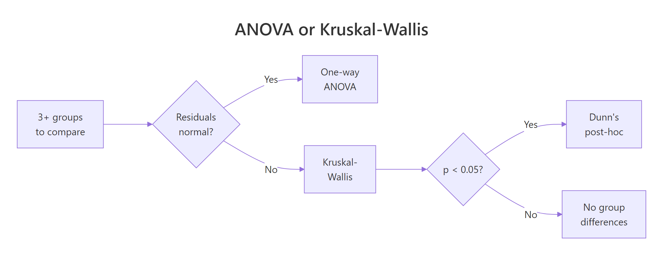
Decision flow: pick ANOVA or Kruskal-Wallis based on residual shape, then proceed to Dunn's post-hoc if the omnibus test is significant.

Figure 1: Decision flow: pick ANOVA or Kruskal-Wallis based on residual shape, then proceed to Dunn's post-hoc if the omnibus test is significant.

A quick boxplot is usually enough to eyeball the third assumption. Groups should have similar spread and similar skew, even if their centres differ.

RBoxplot and sample sizes per group

# Visual check of distribution shape + per-group counts boxplot(weight ~ group, data = pg, main = "PlantGrowth weights by group", ylab = "Dry weight (g)", col = "lightsteelblue") group_sizes <- table(pg$group) group_sizes #> ctrl trt1 trt2 #> 10 10 10

The three boxes have comparable widths and similar whisker lengths, which supports the same-shape assumption. Each group has 10 observations, so the chi-squared approximation for the p-value is safe. If any group dipped below 5 observations, you would set kruskal.test() aside in favour of an exact test via the coin package.

Warning

Without the same-shape assumption, Kruskal-Wallis does not compare medians. It compares stochastic dominance, which is a fancy way of saying "are values from one group systematically larger than values from another?" If one group is heavily skewed and the others are symmetric, a significant test tells you the groups differ somehow, not that their medians differ.

Try it: Report the sample sizes per spray in InsectSprays and check that every group is at least 5.

RYour turn: sample sizes per spray

# Use table() on the spray column ex_sizes <- NULL # your code here ex_sizes #> Expected: 12 observations per spray, so all six groups clear the n >= 5 bar

Click to reveal solution

RInsectSprays sample sizes solution

ex_sizes <- table(InsectSprays$spray) ex_sizes #> A B C D E F #> 12 12 12 12 12 12

Explanation: Every spray has 12 observations, comfortably above the n >= 5 rule of thumb for the chi-squared approximation. No need for an exact test.

How do you measure the Kruskal-Wallis effect size?

A p-value only tells you whether an effect is detectable; it says nothing about whether the effect is big enough to care about. For Kruskal-Wallis, the usual effect size is eta-squared based on H, written $\eta_H^2$. It measures the proportion of variance in ranks explained by group membership, scaled to fall between 0 and 1.

$$\eta_H^2 \;=\; \dfrac{H - k + 1}{n - k}$$

Where:

$H$ = the Kruskal-Wallis statistic you just computed
$k$ = number of groups
$n$ = total observations

Interpret the result with Cohen's thresholds: $\eta_H^2 \approx 0.01$ is a small effect, $0.06$ is medium, $0.14$ and above is large.

RCompute eta-squared-H for PlantGrowth

# Plug H, k, and n into the eta-squared-H formula eta_sq_H <- (H_manual - k + 1) / (n - k) round(eta_sq_H, 3) #> [1] 0.25

An $\eta_H^2$ of 0.25 lands well above Cohen's "large" threshold of 0.14. About a quarter of the variation in the rank of plant weight is attributable to which treatment a plant received. That is a strong effect, worth reporting alongside the p-value in any write-up.

Note

The rstatix::kruskal_effsize() function computes the same number in one call. We compute it by hand here so the code runs anywhere, including inside this browser session. In a local R session, rstatix::kruskal_effsize(pg, weight ~ group) gives the same 0.25 along with a size label and confidence interval.

Try it: Suppose kruskal.test() returned $H = 12.4$ on $k = 4$ groups with $n = 60$ total. Compute $\eta_H^2$.

RYour turn: eta-squared-H from given stats

# Use the formula eta_H^2 = (H - k + 1) / (n - k) ex_H <- 12.4 ex_k <- 4 ex_n <- 60 # your code here: compute and round to 3 decimals ex_eta <- NULL ex_eta #> Expected: about 0.168, a large effect

Click to reveal solution

Reta-squared-H exercise solution

ex_H <- 12.4 ex_k <- 4 ex_n <- 60 ex_eta <- (ex_H - ex_k + 1) / (ex_n - ex_k) round(ex_eta, 3) #> [1] 0.168

Explanation: 0.168 is above Cohen's large-effect cutoff of 0.14, so group membership accounts for a meaningful share of the rank variance.

How do you run Dunn's post-hoc test in R?

A significant Kruskal-Wallis result tells you some group differs, not which pairs. For that you need a post-hoc test that compares every pair of groups and controls the familywise error rate. The classic choice after Kruskal-Wallis is Dunn's test, available in local R sessions as FSA::dunnTest(). Its base-R analogue is pairwise.wilcox.test(), which runs a Wilcoxon rank-sum comparison for each pair and corrects the p-values. We use pairwise.wilcox.test() here because the FSA package is not available in this browser runtime, and the practical conclusions are equivalent.

RPairwise rank-sum tests with Bonferroni correction

# Pairwise comparisons on the same ranked data, Bonferroni-adjusted pairwise_res <- pairwise.wilcox.test(pg$weight, pg$group, p.adjust.method = "bonferroni") pairwise_res #> #> Pairwise comparisons using Wilcoxon rank sum exact test #> #> data: pg$weight and pg$group #> #> ctrl trt1 #> trt1 0.597 - #> trt2 0.537 0.025 #> #> P value adjustment method: bonferroni

Read the matrix as "row vs column": trt1 vs trt2 is the only pair with an adjusted p-value below 0.05. The two fertiliser treatments differ from each other, but neither differs from the control on its own. That matches what the mean-rank table suggested earlier: trt1 pulled weights down, trt2 pushed them up, and the control sat between them.

Tip

Pick the adjustment method to match your situation. "bonferroni" is the most conservative and is fine for a handful of groups. "holm" dominates Bonferroni (same error control, more power) and is a safe default. "BH" (Benjamini-Hochberg) controls the false discovery rate and is preferred when you expect many true differences, as in omics or screening studies.

Try it: Run pairwise rank-sum tests on InsectSprays$count by spray with the Holm adjustment. Which spray pairs differ at the 0.05 level?

RYour turn: pairwise Wilcoxon on InsectSprays

# Same function, different dataset and different adjustment ex_pw <- NULL # your code here ex_pw #> Expected: sprays C, D, E differ from A, B, F; C, D, E do not differ from each other

Click to reveal solution

RInsectSprays pairwise solution

ex_pw <- pairwise.wilcox.test(InsectSprays$count, InsectSprays$spray, p.adjust.method = "holm") ex_pw #> #> Pairwise comparisons using Wilcoxon rank sum test with continuity correction #> #> data: InsectSprays$count and InsectSprays$spray #> #> A B C D E F #> B 1.0000 - - - - - #> C 1.3e-05 2.4e-06 - - - - #> D 5.4e-05 8.3e-06 0.4192 - - - #> E 2.0e-05 5.6e-06 1.0000 1.0000 - - #> F 1.0000 1.0000 2.4e-06 9.6e-06 4.3e-06 - #> #> P value adjustment method: holm

Explanation: Sprays A, B, and F form one high-performance cluster; C, D, and E form a low-performance cluster. Within each cluster, pairs are indistinguishable; between clusters, every pair is highly significant.

How do you report Kruskal-Wallis results?

A clean APA-style line needs five ingredients: the test name, degrees of freedom, the H statistic, the p-value, and the effect size. Readers should be able to reconstruct your analysis from the sentence alone, without hunting through an appendix. Here is a compact template that fits in a single line.

RBuild a one-line APA report string

# sprintf gives you precise control over decimal places apa_line <- sprintf( "Kruskal-Wallis H(%d) = %.2f, p = %.3f, eta-squared-H = %.2f", k - 1, H_manual, kruskal.test(weight ~ group, data = pg)$p.value, eta_sq_H ) apa_line #> [1] "Kruskal-Wallis H(2) = 7.99, p = 0.018, eta-squared-H = 0.25"

Paste that line into a results section and follow it with the pairwise conclusion, for example: "Follow-up pairwise Wilcoxon tests with Bonferroni correction showed that trt1 and trt2 differed significantly (adjusted p = 0.025); neither treatment differed from the control." That is a complete, reproducible, publication-ready summary.

Tip

Always report df, H, p, the effect size, and which pairs drove the difference. A bare "p = 0.018" tells the reader almost nothing. The df anchors how many groups you tested, the effect size says whether the difference matters, and the pairwise breakdown says where the difference lives.

Try it: Given H = 14.2, df = 3, p = 0.0026, and eta-squared-H = 0.18, build the APA report string with sprintf.

RYour turn: APA line from supplied numbers

# Target output: "Kruskal-Wallis H(3) = 14.20, p = 0.003, eta-squared-H = 0.18" ex_H <- 14.2 ex_df <- 3 ex_p <- 0.0026 ex_eta <- 0.18 # your code here: build ex_line with sprintf() ex_line <- NULL ex_line

Click to reveal solution

RAPA line exercise solution

ex_H <- 14.2 ex_df <- 3 ex_p <- 0.0026 ex_eta <- 0.18 ex_line <- sprintf("Kruskal-Wallis H(%d) = %.2f, p = %.3f, eta-squared-H = %.2f", ex_df, ex_H, ex_p, ex_eta) ex_line #> [1] "Kruskal-Wallis H(3) = 14.20, p = 0.003, eta-squared-H = 0.18"

Explanation: %d formats the integer df, %.2f and %.3f fix the decimal places for the statistic and p-value so your results tables look uniform.

Practice Exercises

Exercise 1: Sepal length across iris species

Run a Kruskal-Wallis test on iris$Sepal.Length across iris$Species. Compute the eta-squared-H effect size and decide whether a post-hoc test is warranted. Save the test result to my_iris_kw and the effect size to my_iris_eta.

RExercise 1 starter

# Hint: kruskal.test(Sepal.Length ~ Species, data = iris) # eta_H^2 = (H - k + 1) / (n - k) # Write your code below:

Click to reveal solution

RExercise 1 solution

my_iris_kw <- kruskal.test(Sepal.Length ~ Species, data = iris) print(my_iris_kw) #> #> Kruskal-Wallis rank sum test #> #> data: Sepal.Length by Species #> Kruskal-Wallis chi-squared = 96.937, df = 2, p-value < 2.2e-16 my_iris_H <- unname(my_iris_kw$statistic) my_iris_k <- nlevels(iris$Species) my_iris_n <- nrow(iris) my_iris_eta <- (my_iris_H - my_iris_k + 1) / (my_iris_n - my_iris_k) round(my_iris_eta, 3) #> [1] 0.649

Explanation: The test is highly significant and the effect size (0.65) is enormous, so a pairwise post-hoc is absolutely warranted to say which species pairs drive the difference.

Exercise 2: Full pipeline on chickwts

Build the complete Kruskal-Wallis pipeline for chickwts$weight ~ feed: run the omnibus test, compute eta-squared-H, run pairwise.wilcox.test with Bonferroni, and list which feed pairs differ at the 0.05 level. Save intermediates to my_chicks_kw, my_chicks_eta, and my_chicks_pw.

RExercise 2 starter

# Hint: same steps you just learned, applied to chickwts # Write your code below:

Click to reveal solution

RExercise 2 solution

my_chicks_kw <- kruskal.test(weight ~ feed, data = chickwts) my_chicks_H <- unname(my_chicks_kw$statistic) my_chicks_k <- nlevels(chickwts$feed) my_chicks_n <- nrow(chickwts) my_chicks_eta <- (my_chicks_H - my_chicks_k + 1) / (my_chicks_n - my_chicks_k) round(my_chicks_eta, 3) #> [1] 0.524 my_chicks_pw <- pairwise.wilcox.test(chickwts$weight, chickwts$feed, p.adjust.method = "bonferroni") my_chicks_pw #> #> Pairwise comparisons using Wilcoxon rank sum exact test #> #> data: chickwts$weight and chickwts$feed #> #> casein horsebean linseed meatmeal soybean #> horsebean 1.7e-05 - - - - #> linseed 0.0012 0.0900 - - - #> meatmeal 0.6857 0.0005 0.1108 - - #> soybean 0.0126 0.0063 1.0000 1.0000 - #> sunflower 1.0000 2.6e-05 0.0012 0.8404 0.0055

Explanation: Casein and sunflower are the top performers; horsebean is the worst. Most pairs involving horsebean or sunflower are significant; linseed-soybean and meatmeal-soybean are not. Eta-squared-H of 0.52 is a very large effect.

Exercise 3: Compute H from scratch

Given a numeric vector my_vals and a factor my_grp, compute the Kruskal-Wallis H statistic without calling kruskal.test, then verify it matches what kruskal.test returns. Use the formula $H = \dfrac{12}{N(N+1)} \sum R_i^2 / n_i - 3(N+1)$.

RExercise 3 starter

set.seed(42) my_vals <- c(rnorm(8, 5), rnorm(8, 6), rnorm(8, 7)) my_grp <- factor(rep(c("A", "B", "C"), each = 8)) # Write your code below to compute my_H_scratch

Click to reveal solution

RExercise 3 solution

set.seed(42) my_vals <- c(rnorm(8, 5), rnorm(8, 6), rnorm(8, 7)) my_grp <- factor(rep(c("A", "B", "C"), each = 8)) my_ranks <- rank(my_vals) my_R <- tapply(my_ranks, my_grp, sum) my_ni <- table(my_grp) my_N <- length(my_vals) my_H_scratch <- (12 / (my_N * (my_N + 1))) * sum(my_R^2 / my_ni) - 3 * (my_N + 1) round(my_H_scratch, 4) #> [1] 13.79 # Check against kruskal.test round(unname(kruskal.test(my_vals, my_grp)$statistic), 4) #> [1] 13.79

Explanation: The two values match to four decimals, confirming the formula. kruskal.test() applies a small tie-correction when ranks are tied, so for continuous data with no ties the manual and built-in answers are identical.

Complete Example

Here is the full pipeline applied end-to-end to the airquality dataset, which records daily ozone in parts per billion across five months. Ozone is notoriously right-skewed, making it an almost textbook use case for Kruskal-Wallis.

REnd-to-end Kruskal-Wallis on airquality

# Prepare the data: drop missing ozone values and make Month a factor aq <- airquality[!is.na(airquality$Ozone), ] aq$Month <- factor(aq$Month, levels = 5:9, labels = c("May", "Jun", "Jul", "Aug", "Sep")) # Shape check: boxplot makes the skew obvious boxplot(Ozone ~ Month, data = aq, col = "lightsteelblue", main = "Daily ozone by month", ylab = "Ozone (ppb)") # Omnibus test aq_kw <- kruskal.test(Ozone ~ Month, data = aq) aq_kw #> #> Kruskal-Wallis rank sum test #> #> data: Ozone by Month #> Kruskal-Wallis chi-squared = 29.267, df = 4, p-value = 6.901e-06 # Effect size aq_H <- unname(aq_kw$statistic) aq_k <- nlevels(aq$Month) aq_n <- nrow(aq) aq_eta <- (aq_H - aq_k + 1) / (aq_n - aq_k) round(aq_eta, 3) #> [1] 0.225 # Post-hoc pairwise comparisons aq_pairs <- pairwise.wilcox.test(aq$Ozone, aq$Month, p.adjust.method = "bonferroni") aq_pairs #> #> Pairwise comparisons using Wilcoxon rank sum test with continuity correction #> #> data: aq$Ozone and aq$Month #> #> May Jun Jul Aug #> Jun 1.00000 - - - #> Jul 0.00014 0.00377 - - #> Aug 0.00026 0.00511 1.00000 - #> Sep 1.00000 1.00000 0.00677 0.01392 # One-line APA report aq_report <- sprintf( "Kruskal-Wallis H(%d) = %.2f, p = %.4f, eta-squared-H = %.2f", aq_k - 1, aq_H, aq_kw$p.value, aq_eta ) aq_report #> [1] "Kruskal-Wallis H(4) = 29.27, p = 0.0000, eta-squared-H = 0.22"

The omnibus test rejects equality of monthly ozone distributions with a p-value around 7e-06. The effect size of 0.22 is large by Cohen's thresholds, so the month-to-month difference is practically meaningful. The pairwise matrix shows the shape of the pattern: July and August are indistinguishable from each other but significantly higher than May, June, and September. In plain English, the two summer months carry elevated ozone, which matches the well-known photochemistry of hot, sunny weather driving ground-level ozone formation.

Summary

The Kruskal-Wallis test is the go-to tool when you want to compare three or more independent groups but cannot trust ANOVA's assumptions. Ranks replace raw values, so skew and heavy tails stop mattering, and the test stays valid on small samples.

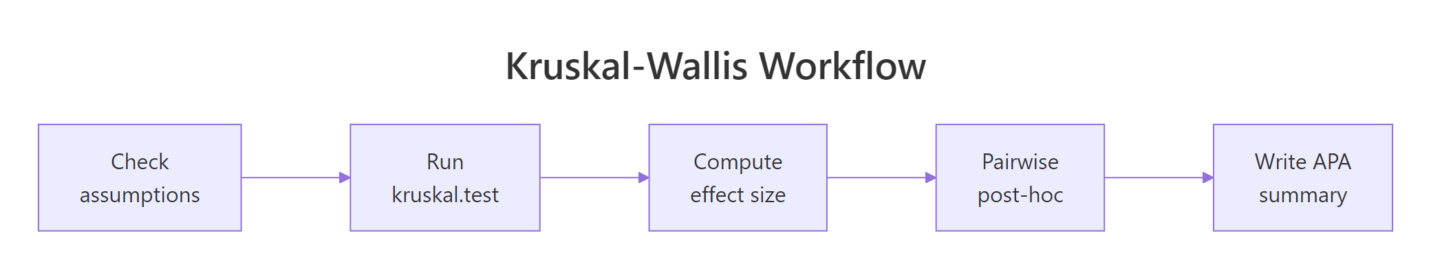
The five-step Kruskal-Wallis analysis workflow from assumption checks through reporting.

Figure 2: The five-step Kruskal-Wallis analysis workflow from assumption checks through reporting.

Step	Function	What it tells you
Check assumptions	`boxplot()`, `table()`	Are groups independent and similar in shape? Is every group n ≥ 5?
Run the omnibus test	`kruskal.test(y ~ g)`	Does any group differ from the others?
Compute effect size	$(H - k + 1) / (n - k)$	How strong is the difference? Small, medium, or large?
Pairwise post-hoc	`pairwise.wilcox.test()`	Which specific pairs drive the omnibus result?
Report results	`sprintf()`	One APA-style line with df, H, p, effect size.

References

Kruskal, W. H. & Wallis, W. A. (1952). Use of ranks in one-criterion variance analysis. Journal of the American Statistical Association 47(260), 583-621. Link
Dunn, O. J. (1964). Multiple comparisons using rank sums. Technometrics 6(3), 241-252. Link
R Core Team. ?kruskal.test documentation. Link
R Core Team. ?pairwise.wilcox.test documentation. Link
Tomczak, M. & Tomczak, E. (2014). The need to report effect size estimates revisited. Trends in Sport Sciences 1(21), 19-25.
Mangiafico, S. (2016). R Companion Handbook: Kruskal-Wallis Test. Link
rstatix::kruskal_effsize() reference. Link
Hollander, M., Wolfe, D. A., & Chicken, E. (2014). Nonparametric Statistical Methods, 3rd ed. Wiley. Chapter 6.

Continue Learning

One-Way ANOVA in R, the parametric sibling of this test, covering F-statistics, Levene's test, and Tukey's HSD.
Welch's ANOVA in R, for use when variances are unequal but the data is still approximately normal.
Wilcoxon Rank-Sum Test in R, the two-sample rank test, which Kruskal-Wallis generalises to three or more groups.

Kruskal-Wallis Test in R: One-Way Nonparametric ANOVA with Post-Hoc

When should you use the Kruskal-Wallis test instead of ANOVA?

How does the Kruskal-Wallis test work with ranks?

What are the assumptions of the Kruskal-Wallis test?

How do you measure the Kruskal-Wallis effect size?

How do you run Dunn's post-hoc test in R?

How do you report Kruskal-Wallis results?

Practice Exercises

Exercise 1: Sepal length across iris species

Exercise 2: Full pipeline on chickwts

Exercise 3: Compute H from scratch

Complete Example

Summary

References

Continue Learning

Related Tutorials