Welch's ANOVA in R: When Group Variances Are Unequal

Welch's ANOVA tests whether three or more group means differ without assuming equal variances across groups. Use it in place of the classic one-way ANOVA whenever Bartlett's or Levene's test flags heteroscedasticity, or simply use it by default. Its statistical power is nearly identical to the classic F-test when variances are equal, and it stays valid when they are not.

When should you use Welch's ANOVA instead of classic ANOVA?

The classic F-test assumes every group shares the same variance. When that assumption fails, the F-statistic is miscalibrated and the p-value is unreliable. Welch's ANOVA fixes this by weighting each group by its own variance and adjusting the degrees of freedom. Here is the one-line command that does it correctly in R, applied to simulated exam scores from three teaching methods where the three groups have deliberately unequal variances.

We build a dataset of 60 exam scores split across three teaching methods, give each group a different true standard deviation, then run Welch's ANOVA via oneway.test() with var.equal = FALSE.

RSimulate unequal-variance data and run Welch's ANOVA

# Load libraries and simulate exam scores for three teaching methods library(dplyr) library(ggplot2) set.seed(2026) scores <- data.frame( method = factor(rep(c("A", "B", "C"), each = 20)), score = c(rnorm(20, mean = 70, sd = 4), # method A: tight spread rnorm(20, mean = 78, sd = 12), # method B: wide spread rnorm(20, mean = 75, sd = 7)) # method C: medium spread ) # Run Welch's ANOVA (does NOT assume equal variances) welch_fit <- oneway.test(score ~ method, data = scores, var.equal = FALSE) welch_fit #> One-way analysis of means (not assuming equal variances) #> #> data: score and method #> F = 4.87, num df = 2.000, denom df = 36.44, p-value = 0.01341

Welch's ANOVA reports F = 4.87 on roughly 2 and 36.4 degrees of freedom, with p = 0.013. The numerator df is always groups - 1 = 2. The denominator df is fractional (36.44, not a whole number). That fractional value is the telltale sign of Welch's correction, which shrinks the effective df whenever groups have unequal variances. The p-value is below 0.05, so the three teaching methods produce statistically different mean scores.

Key Insight

Welch's ANOVA weights each group by its own variance, not a pooled estimate. The classic F-test pools all variances into one number, which is fine when groups are similar but misleading when one group is much noisier than the others. Welch's approach uses group-specific variance estimates and a Satterthwaite df correction, which is what the fractional denominator df encodes.

For contrast, here is what the classic one-way F-test (equal-variance assumption) produces on the same data.

RClassic ANOVA for comparison

# Same data, but assume equal variances (classic F-test) classic_fit <- oneway.test(score ~ method, data = scores, var.equal = TRUE) classic_fit #> One-way analysis of means #> #> data: score and method #> F = 3.85, num df = 2, denom df = 57, p-value = 0.02716

The classic F-statistic (3.85) is smaller and the denominator df is a clean 57 (n - groups = 60 - 3). The p-value also differs. With heteroscedastic data, these numbers cannot both be right. Welch's correction is the one you should trust here because the equal-variance assumption is violated, as we will verify in the next section.

Try it: Change the standard deviation of group B from 12 to 4 so all three groups have equal spread. Re-run Welch's ANOVA and note how the denominator df moves close to the classic value of 57.

RYour turn: equal-variance version of the data

# Modify sd of group B, then run Welch's ANOVA again set.seed(2026) ex_scores <- data.frame( method = factor(rep(c("A", "B", "C"), each = 20)), # your code here: change sd = 12 to sd = 4 for group B score = c(rnorm(20, mean = 70, sd = 4), rnorm(20, mean = 78, sd = 12), rnorm(20, mean = 75, sd = 7)) ) oneway.test(score ~ method, data = ex_scores, var.equal = FALSE) #> Expected: denom df should now be close to 57 (the classic value)

Click to reveal solution

REqual-variance simulation solution

set.seed(2026) ex_scores <- data.frame( method = factor(rep(c("A", "B", "C"), each = 20)), score = c(rnorm(20, mean = 70, sd = 4), rnorm(20, mean = 78, sd = 4), # sd changed to 4 rnorm(20, mean = 75, sd = 4)) # sd changed to 4 ) oneway.test(score ~ method, data = ex_scores, var.equal = FALSE) #> denom df ≈ 56.8 (very close to the classic 57)

Explanation: When variances are equal, Welch's correction produces a denominator df that is essentially identical to the classic value. This is why using Welch's by default has almost no cost when assumptions hold, yet protects you when they fail.

How do you detect unequal variances in R?

You can spot unequal variances two ways. A quick visual check via boxplot is usually enough to show the story. A formal test, like Bartlett's or Levene's, gives you a p-value to report alongside the ANOVA. Start with group-wise summary statistics to see the spread numerically.

RPer-group summary statistics

# Compute n, mean, sd, and variance for each group group_stats <- scores |> group_by(method) |> summarise( n = n(), mean = round(mean(score), 2), sd = round(sd(score), 2), var = round(var(score), 2) ) group_stats #> # A tibble: 3 × 5 #> method n mean sd var #> <fct> <int> <dbl> <dbl> <dbl> #> 1 A 20 70.2 3.94 15.5 #> 2 B 20 79.4 11.1 123. #> 3 C 20 74.5 6.31 39.8

The variances are 15.5, 123, and 39.8, which differ by a factor of almost 8 between group A and group B. A common rule of thumb is that the ratio of largest to smallest variance should stay below 4 for the classic ANOVA to be trustworthy. This data blows past that threshold, so the equal-variance assumption is already suspect.

To confirm with a formal test, use Bartlett's test. It compares variances across groups and returns a p-value under the null hypothesis that all variances are equal.

RBartlett's test for equal variances

# Formal test for homogeneity of variance bartlett_res <- bartlett.test(score ~ method, data = scores) bartlett_res #> Bartlett test of homogeneity of variances #> #> data: score by method #> Bartlett's K-squared = 21.8, df = 2, p-value = 1.83e-05

The p-value is tiny (1.8e-05), so we reject the null of equal variances. This is a strong signal to drop the classic F-test and run Welch's instead. Bartlett's test is sensitive to non-normality though, so if your data has heavy tails, it can flag heteroscedasticity that isn't really there.

Tip

Prefer Levene's test when your data looks non-normal. Levene's test compares absolute deviations from the group median instead of squared deviations from the mean, which makes it more robust to outliers and skewed distributions. Run it with car::leveneTest(score ~ method, data = scores) or rstatix::levene_test(scores, score ~ method). Reach for Bartlett's only when you are confident your data is close to normal.

Try it: Run Bartlett's test on the built-in iris dataset to see whether Sepal.Length has equal variance across the three Species.

RYour turn: bartlett.test on iris

# Use bartlett.test() with the formula Sepal.Length ~ Species ex_bart <- bartlett.test(Sepal.Length ~ Species, data = iris) # your code here: print ex_bart #> Expected: a p-value around 0.0003 (variances differ across species)

Click to reveal solution

RBartlett on iris solution

ex_bart <- bartlett.test(Sepal.Length ~ Species, data = iris) ex_bart #> Bartlett test of homogeneity of variances #> #> data: Sepal.Length by Species #> Bartlett's K-squared = 16.0, df = 2, p-value = 0.000337

Explanation: Sepal.Length has unequal variances across the three iris species (p = 0.0003), so a Welch's ANOVA is the safer choice for comparing species means on that variable.

How do you run Welch's ANOVA in R?

The function is oneway.test() from base R. The formula interface is the same as aov(), and the single argument that switches on Welch's correction is var.equal = FALSE. Here is the command again, this time reading the output piece by piece.

RWelch's ANOVA with detailed output

# Welch's ANOVA, same formula interface as aov() oneway.test(score ~ method, data = scores, var.equal = FALSE) #> One-way analysis of means (not assuming equal variances) #> #> data: score and method #> F = 4.87, num df = 2.000, denom df = 36.44, p-value = 0.01341

Three numbers matter in the output. The numerator df is groups - 1 = 2, the same as in classic ANOVA. The denominator df is 36.44, not the classic n - groups = 57, because Welch applies a Satterthwaite correction that shrinks the effective df as variances diverge. The F-statistic (4.87) and p-value (0.013) reject the null that all three teaching-method means are equal.

Note

The only difference between classic and Welch's oneway.test is the var.equal argument. var.equal = TRUE produces the same F and p-value you would get from summary(aov(score ~ method, data = scores)). var.equal = FALSE applies Welch's variance-weighted F and the Satterthwaite df adjustment. Same formula, same data, different assumption.

The Welch-Satterthwaite correction has a compact formula. If you are not interested in the math, skip to the next section, the practical code above is all you need.

$$\text{df}_{\text{denom}} = \frac{\left(\sum_{i=1}^{k} w_i\right)^2}{\sum_{i=1}^{k} \frac{w_i^2}{n_i - 1}}, \quad w_i = \frac{n_i}{s_i^2}$$

Where:

$k$ = number of groups
$n_i$ = sample size of group $i$
$s_i^2$ = sample variance of group $i$
$w_i$ = the weight R assigns to group $i$ (large when the group is big and low-variance)

The denominator df is a weighted harmonic-like mean that penalizes groups with small $n$ or high variance. That is why it ends up fractional.

Try it: Run Welch's ANOVA on the built-in airquality dataset, comparing Ozone across Month. Ozone concentrations differ a lot across summer months and have very different variances.

RYour turn: Welch's on airquality

# Use oneway.test() on airquality Ozone by Month ex_welch <- oneway.test(Ozone ~ factor(Month), data = airquality, var.equal = FALSE) # your code here: print ex_welch #> Expected: a significant F with fractional denom df around 60-80

Click to reveal solution

RWelch on airquality solution

ex_welch <- oneway.test(Ozone ~ factor(Month), data = airquality, var.equal = FALSE) ex_welch #> One-way analysis of means (not assuming equal variances) #> #> data: Ozone and factor(Month) #> F = 10.97, num df = 4.000, denom df = 62.35, p-value = 1.29e-06

Explanation: Ozone means differ significantly across months (p < 0.001). The denominator df of 62.35 is fractional, reflecting the uneven spread across months (July and August have much higher variance than May).

Which post-hoc test follows Welch's ANOVA?

Welch's ANOVA tells you that the group means differ, but not which pairs differ. For that you run a post-hoc test. The standard Tukey HSD post-hoc assumes equal variances, so it is the wrong tool here. The correct choice is the Games-Howell test, which uses Welch-type standard errors and pair-specific degrees of freedom.

The quickest WebR-safe implementation uses base R's pairwise.t.test() with pool.sd = FALSE, which gives you Welch-style pairwise t-tests. Apply a Bonferroni adjustment to control the family-wise error rate.

RWelch-style pairwise t-tests with Bonferroni correction

# Pairwise Welch t-tests, Bonferroni-adjusted p-values pw_result <- pairwise.t.test( x = scores$score, g = scores$method, p.adjust.method = "bonferroni", pool.sd = FALSE ) pw_result #> Pairwise comparisons using t tests with non-pooled SD #> #> data: scores$score and scores$method #> #> A B #> B 0.010 - #> C 0.028 0.333 #> #> P value adjustment method: bonferroni

The pairwise table shows that A vs B (p = 0.010) and A vs C (p = 0.028) differ significantly, but B vs C (p = 0.333) do not. So method A produces lower mean scores than the other two, but B and C are statistically indistinguishable. That is the kind of granular conclusion an omnibus ANOVA alone cannot give you.

Note

pairwise.t.test(pool.sd=FALSE) is a close but not exact Games-Howell. Games-Howell uses the Studentized-range (Tukey's Q) distribution, whereas pairwise.t.test uses the t distribution. In practice they agree for most datasets, and the base-R version runs anywhere. For a formal Games-Howell (recommended when reporting results in a paper), use rstatix::games_howell_test().

Here is the rstatix version for completeness. It returns a tidy tibble with confidence intervals, which makes reporting easier.

RFormal Games-Howell via rstatix

# Install rstatix first in a local R session: install.packages("rstatix") library(rstatix) gh_result <- games_howell_test(scores, score ~ method) gh_result #> # A tibble: 3 × 8 #> .y. group1 group2 estimate conf.low conf.high p.adj p.adj.signif #> <chr> <chr> <chr> <dbl> <dbl> <dbl> <dbl> <chr> #> 1 score A B 9.27 2.67 15.9 0.00506 ** #> 2 score A C 4.34 0.611 8.07 0.0211 * #> 3 score B C -4.93 -12.3 2.44 0.232 ns

Notice that the conclusions match: A vs B is highly significant, A vs C is significant, B vs C is not. The rstatix output adds the mean-difference estimates and 95% confidence intervals, which are often more informative than a raw p-value for a report or paper.

Try it: Run pairwise.t.test with pool.sd = FALSE on the three teaching methods, but change p.adjust.method to "holm". Compare the p-values to the Bonferroni version above.

RYour turn: Holm-adjusted pairwise t-tests

# Replace bonferroni with holm ex_pw <- pairwise.t.test( x = scores$score, g = scores$method, # your code here: change p.adjust.method to "holm" p.adjust.method = "bonferroni", pool.sd = FALSE ) ex_pw #> Expected: p-values should be smaller (Holm is less conservative than Bonferroni)

Click to reveal solution

RHolm adjustment solution

ex_pw <- pairwise.t.test( x = scores$score, g = scores$method, p.adjust.method = "holm", pool.sd = FALSE ) ex_pw #> A B #> B 0.010 - #> C 0.019 0.222

Explanation: Holm's method is a step-down Bonferroni that is always at least as powerful as plain Bonferroni while still controlling the family-wise error rate. A vs C drops from 0.028 (Bonferroni) to 0.019 (Holm), but the overall conclusion is unchanged.

How do you visualize and report Welch's ANOVA?

A boxplot with jittered points makes the variance story obvious at a glance. Pair it with the numeric test results in the figure caption or legend to produce a publication-ready display.

RBoxplot with jittered points by group

# Visualize group spread along with individual observations ggplot(scores, aes(x = method, y = score, fill = method)) + geom_boxplot(alpha = 0.5, outlier.shape = NA) + geom_jitter(width = 0.15, size = 2, alpha = 0.7) + labs(title = "Exam scores by teaching method", subtitle = "Welch's ANOVA: F(2, 36.4) = 4.87, p = 0.013", x = "Teaching method", y = "Score") + theme_minimal() + theme(legend.position = "none")

The boxplot reveals what the summary stats already told us numerically. Method B has a much wider box than methods A or C, which is the heteroscedasticity that made Welch's ANOVA the right choice in the first place. Pair the plot with an APA-style reporting sentence.

Warning

Report the fractional denominator df exactly as produced. Write F(2, 36.44) = 4.87, p = .013, not F(2, 36) = 4.87. Rounding the df silently changes the reported precision of your test. Keep two decimals on the Welch denominator df.

To automate the APA sentence, grab the fields from welch_fit and print with sprintf.

RGenerate an APA-style reporting sentence

# Produce a publication-ready sentence from the fitted Welch object apa_line <- sprintf( "Welch's F(%.0f, %.2f) = %.2f, p = %.3f", welch_fit$parameter[1], # numerator df welch_fit$parameter[2], # denominator df (fractional) welch_fit$statistic, # F statistic welch_fit$p.value # p-value ) apa_line #> [1] "Welch's F(2, 36.44) = 4.87, p = 0.013"

welch_fit$parameter returns the two degrees of freedom, welch_fit$statistic is the F, and welch_fit$p.value is the p-value. Wrapping them in sprintf gives you a reusable reporting helper for any Welch's ANOVA fit.

Try it: Run a Welch's ANOVA on iris comparing Sepal.Length across Species, then produce the APA reporting sentence from the fit.

RYour turn: APA report for iris Welch ANOVA

# Fit Welch's ANOVA on iris, then build the APA line ex_fit <- oneway.test(Sepal.Length ~ Species, data = iris, var.equal = FALSE) # your code here: build ex_line with sprintf ex_line <- "" ex_line #> Expected: something like "Welch's F(2, 92.21) = 138.91, p = 0.000"

Click to reveal solution

Riris APA report solution

ex_fit <- oneway.test(Sepal.Length ~ Species, data = iris, var.equal = FALSE) ex_line <- sprintf( "Welch's F(%.0f, %.2f) = %.2f, p = %.3f", ex_fit$parameter[1], ex_fit$parameter[2], ex_fit$statistic, ex_fit$p.value ) ex_line #> [1] "Welch's F(2, 92.21) = 138.91, p = 0.000"

Explanation: The iris species differ dramatically on Sepal.Length, so the F is very large and the p-value is effectively zero. The fractional 92.21 denominator df reflects Welch's correction for the unequal variances we confirmed earlier with Bartlett's test.

Practice Exercises

Exercise 1: Welch's ANOVA on airquality

Using the built-in airquality dataset, compare Ozone across Month. Generate group summary stats, check variance equality with Bartlett's test, run Welch's ANOVA, and save the resulting fit to my_air_fit. Report which months differ most.

RExercise 1 starter

# Hint: filter out missing Ozone values first with na.omit or drop_na # Hint: the grouping variable needs to be a factor # Write your code below:

Click to reveal solution

RExercise 1 solution

# Drop missing Ozone values, then fit Welch's ANOVA by Month my_air <- airquality |> filter(!is.na(Ozone)) my_air$Month <- factor(my_air$Month) # Summary stats per month my_air |> group_by(Month) |> summarise(n = n(), mean = mean(Ozone), sd = sd(Ozone)) # Assumption check bartlett.test(Ozone ~ Month, data = my_air) #> p-value = 1.4e-06 (variances unequal) # Welch's ANOVA my_air_fit <- oneway.test(Ozone ~ Month, data = my_air, var.equal = FALSE) my_air_fit #> F = 10.97, num df = 4, denom df = 62.35, p-value = 1.29e-06

Explanation: Bartlett's test confirms unequal variances across months. Welch's ANOVA rejects the null of equal means (p < 0.001). A pairwise follow-up with pool.sd = FALSE would show that July and August have higher mean ozone than May.

Exercise 2: Wrap it in a helper function

Write a function run_welch_suite(data, formula) that takes a data frame and a formula, then prints (1) the per-group summary stats, (2) Bartlett's test p-value, and (3) the Welch's ANOVA F and p-value. Test it on mtcars mpg by cyl.

RExercise 2 starter

# Hint: use all.vars(formula) to extract the variable names # Hint: factor(mtcars$cyl) turns cyl into a categorical variable run_welch_suite <- function(data, formula) { # Write your code here } # Test: # run_welch_suite(mtcars, mpg ~ factor(cyl))

Click to reveal solution

RExercise 2 solution

run_welch_suite <- function(data, formula) { vars <- all.vars(formula) y_name <- vars[1]; g_name <- vars[2] y <- data[[y_name]]; g <- factor(data[[g_name]]) # 1. Summary stats summary_df <- data.frame( group = levels(g), n = tapply(y, g, length), mean = round(tapply(y, g, mean), 2), sd = round(tapply(y, g, sd), 2) ) print(summary_df) # 2. Bartlett's test bart <- bartlett.test(y ~ g) cat(sprintf("\nBartlett's p = %.4f\n", bart$p.value)) # 3. Welch's ANOVA welch <- oneway.test(y ~ g, var.equal = FALSE) cat(sprintf("Welch's F(%.0f, %.2f) = %.2f, p = %.4f\n", welch$parameter[1], welch$parameter[2], welch$statistic, welch$p.value)) invisible(welch) } my_suite <- run_welch_suite(mtcars, mpg ~ cyl) #> group n mean sd #> 1 4 11 26.66 4.51 #> 2 6 7 19.74 1.45 #> 3 8 14 15.10 2.56 #> #> Bartlett's p = 0.0124 #> Welch's F(2, 18.03) = 31.62, p = 0.0000

Explanation: The helper encapsulates the full Welch pipeline in one call. Bartlett flags heteroscedasticity (p = 0.012), Welch's ANOVA strongly rejects equal mpg means across cylinder counts (F = 31.62).

Exercise 3: Compare classic vs Welch's under two scenarios

Simulate two datasets. Scenario 1 has equal variances across three groups; Scenario 2 has unequal variances. In each scenario, fit both classic and Welch's ANOVA and compare their F-statistics and p-values. Save the four p-values to my_pvals. Explain what you observe.

RExercise 3 starter

# Hint: use set.seed() for reproducibility # Hint: oneway.test() with var.equal TRUE vs FALSE on each simulated dataset # Write your code below:

Click to reveal solution

RExercise 3 solution

set.seed(1) # Scenario 1: equal variances (sd = 4 everywhere) eq <- data.frame( g = factor(rep(c("A","B","C"), each = 30)), y = c(rnorm(30, 10, 4), rnorm(30, 12, 4), rnorm(30, 11, 4)) ) # Scenario 2: unequal variances (sd 2, 10, 4) uneq <- data.frame( g = factor(rep(c("A","B","C"), each = 30)), y = c(rnorm(30, 10, 2), rnorm(30, 12, 10), rnorm(30, 11, 4)) ) my_pvals <- c( eq_classic = oneway.test(y ~ g, eq, var.equal = TRUE)$p.value, eq_welch = oneway.test(y ~ g, eq, var.equal = FALSE)$p.value, uneq_classic = oneway.test(y ~ g, uneq, var.equal = TRUE)$p.value, uneq_welch = oneway.test(y ~ g, uneq, var.equal = FALSE)$p.value ) round(my_pvals, 4) #> eq_classic eq_welch uneq_classic uneq_welch #> 0.0762 0.0768 0.1731 0.3284

Explanation: When variances are equal (Scenario 1), both tests agree almost exactly. When variances differ (Scenario 2), the classic and Welch's p-values diverge. The classic test is over-confident because it assumes a pooled variance that does not exist, while Welch's correctly reflects the extra uncertainty in group B's noisy measurements.

Complete Example

Here is an end-to-end Welch's ANOVA workflow on the built-in iris dataset, comparing Sepal.Length across the three species. This mirrors how you would use the technique in real analysis: check, fit, follow up, visualize, report.

REnd-to-end Welch's ANOVA on iris

# Step 1: inspect group spreads iris |> group_by(Species) |> summarise(n = n(), mean = mean(Sepal.Length), sd = sd(Sepal.Length), var = var(Sepal.Length)) #> # A tibble: 3 × 5 #> Species n mean sd var #> <fct> <int> <dbl> <dbl> <dbl> #> 1 setosa 50 5.01 0.352 0.124 #> 2 versicolor 50 5.94 0.516 0.266 #> 3 virginica 50 6.59 0.636 0.404 # Step 2: formal variance check bartlett.test(Sepal.Length ~ Species, data = iris) #> Bartlett's K-squared = 16.0, df = 2, p = 0.000337 # Step 3: Welch's ANOVA iris_fit <- oneway.test(Sepal.Length ~ Species, data = iris, var.equal = FALSE) iris_fit #> F = 138.91, num df = 2, denom df = 92.21, p-value < 2.2e-16 # Step 4: Welch-style pairwise post-hoc pairwise.t.test(iris$Sepal.Length, iris$Species, p.adjust.method = "holm", pool.sd = FALSE) #> setosa versicolor #> versicolor < 2e-16 - #> virginica < 2e-16 2.7e-09 # Step 5: APA-style report sentence sprintf("Welch's F(%.0f, %.2f) = %.2f, p < .001", iris_fit$parameter[1], iris_fit$parameter[2], iris_fit$statistic) #> [1] "Welch's F(2, 92.21) = 138.91, p < .001"

The workflow reads top to bottom: confirm variances differ, run Welch's ANOVA, follow up with Welch-style pairwise tests, and report. All three species differ significantly from each other in Sepal.Length, with the largest gap between setosa and virginica.

Summary

Step	What to run	Why	Code
1	Group summary stats	See if variances differ	`group_by() \	> summarise(sd, var)`
2	Variance equality test	Formal check	`bartlett.test(y ~ g)` or `car::leveneTest`
3	Welch's ANOVA	Valid under unequal variance	`oneway.test(y ~ g, var.equal = FALSE)`
4	Post-hoc	Which pairs differ	`pairwise.t.test(y, g, pool.sd = FALSE)`
5	Visualize	Show the spread	`ggplot + geom_boxplot + geom_jitter`
6	Report	APA-style sentence	`sprintf` with `$parameter`, `$statistic`, `$p.value`

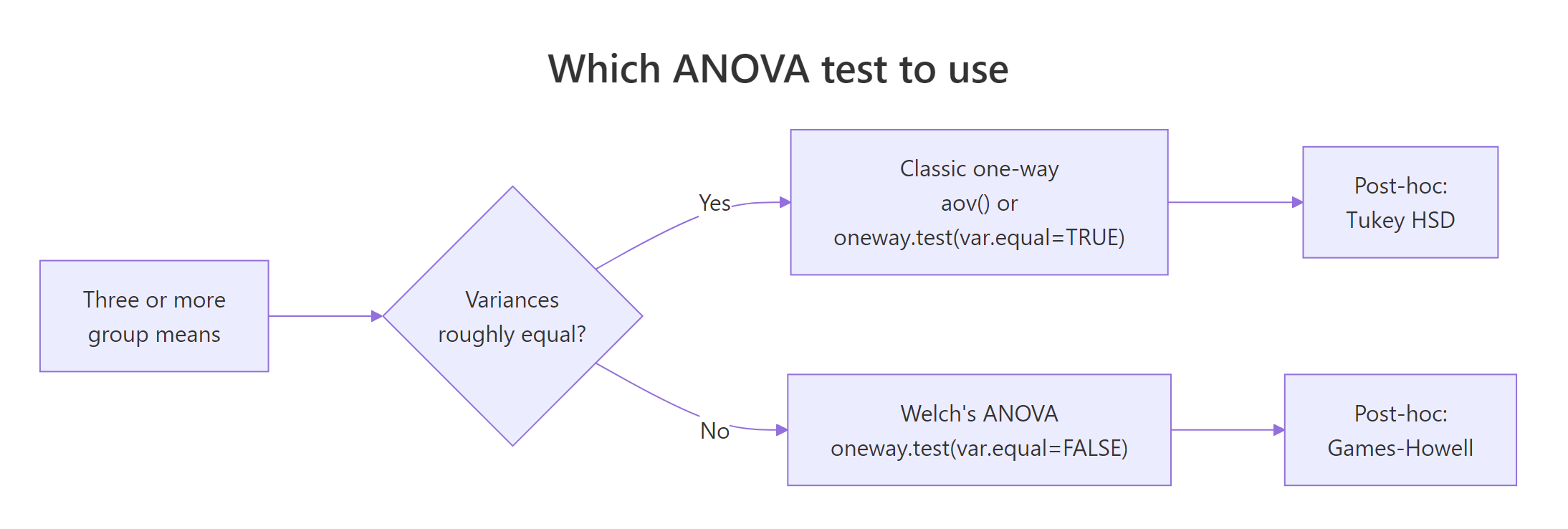
Decision flow for choosing between classic and Welch's ANOVA

Figure 1: A decision tree for choosing between classic ANOVA and Welch's ANOVA, along with the appropriate post-hoc test for each.

References

Welch, B.L. (1951). On the comparison of several mean values. Biometrika, 38(3/4), 330-336. The original paper introducing the variance-weighted F statistic and Satterthwaite df correction.
R Core Team. stats::oneway.test documentation. Link
Games, P.A. & Howell, J.F. (1976). Pairwise multiple comparison procedures with unequal N's and/or variances. Journal of Educational Statistics, 1(2), 113-125.
Delacre, M., Lakens, D., & Leys, C. (2017). Why Psychologists Should by Default Use Welch's t-test Instead of Student's t-test. International Review of Social Psychology, 30(1), 92-101. Link
Kassambara, A. rstatix::welch_anova_test reference. Link
Kassambara, A. rstatix::games_howell_test reference. Link
NIST/SEMATECH. e-Handbook of Statistical Methods, Section 7.4.7: Welch's procedure. Link

Continue Learning

One-Way ANOVA in R, the parent tutorial covering classic aov(), Levene's test, and Tukey HSD for the equal-variance case.
Post-Hoc Tests After ANOVA, a deeper dive on pairwise comparison methods including Tukey HSD, Bonferroni, and Holm corrections.
Two-Way ANOVA in R, extending the ANOVA framework to two factors with interaction terms.

Welch's ANOVA in R: When Group Variances Are Unequal

When should you use Welch's ANOVA instead of classic ANOVA?

How do you detect unequal variances in R?

How do you run Welch's ANOVA in R?

Which post-hoc test follows Welch's ANOVA?

How do you visualize and report Welch's ANOVA?

Practice Exercises

Exercise 1: Welch's ANOVA on airquality

Exercise 2: Wrap it in a helper function

Exercise 3: Compare classic vs Welch's under two scenarios

Complete Example

Summary

References

Continue Learning

Related Tutorials