ggplot2 + plotly: Add Hover Tooltips and Zoom to Any Chart in One Line

ggplotly() converts any ggplot2 chart into an interactive plotly widget with hover tooltips, zoom, pan, and click-to-filter — in a single function call.

How Does ggplotly() Turn a Static Chart Interactive?

You have a polished ggplot2 scatter plot and your stakeholder asks "can I hover over the points to see which car that is?" With base ggplot2, the answer is a flat PNG. With plotly, the answer is one function call. ggplotly() reads every aesthetic, axis, and layer from your ggplot object and rebuilds it as a JavaScript widget the reader can explore.

library(ggplot2) library(plotly) p <- ggplot(mpg, aes(x = displ, y = hwy, color = class)) + geom_point(size = 2) + labs(title = "Engine Size vs Highway Mileage", x = "Displacement (L)", y = "Highway MPG") p #> A scatter plot with 234 points colored by vehicle class #> Larger engines cluster at lower highway MPG

That static chart already tells a story. Now make it interactive with a single line.

ggplotly(p) #> An interactive plotly widget: #> - Hover over any point to see class, displ, and hwy #> - Click-drag to zoom into a region #> - Double-click to reset the view #> - Click legend entries to show/hide a class

Every aesthetic you mapped in ggplot2 — colour, size, shape — carries over. The tooltip shows those mapped values by default, and the toolbar in the top-right corner lets users zoom, pan, and download the chart as a PNG.

Note

Interactive plotly output renders in RStudio and HTML documents, not in the browser code runner. The code blocks here run the R code and show text output. Copy the code into RStudio or an R Markdown document to see the full interactive chart with hover, zoom, and click features.

Try it: Build a bar chart counting the number of cars per class in mpg using geom_bar(), then convert it with ggplotly().

# Try it: bar chart → interactive ex_bar <- ggplot(mpg, aes(x = class)) + geom_bar(fill = "steelblue") + labs(title = "Cars by Class") # Convert to interactive: # your code here

Click to reveal solution

ex_bar <- ggplot(mpg, aes(x = class)) + geom_bar(fill = "steelblue") + labs(title = "Cars by Class") ggplotly(ex_bar) #> Interactive bar chart — hover over each bar to see the count

Explanation: ggplotly() works on any ggplot2 object, including bar charts. Hover shows the x category and count.

How Do You Control What Appears in the Tooltip?

By default, ggplotly() shows every mapped aesthetic in the tooltip — x, y, colour, size, and anything else in aes(). That's often too much. The tooltip argument lets you pick exactly which aesthetics appear.

Let's start by limiting the tooltip to just the x and y values.

p2 <- ggplot(mpg, aes(x = displ, y = hwy, color = class)) + geom_point(size = 2) + labs(x = "Displacement (L)", y = "Highway MPG") ggplotly(p2, tooltip = c("x", "y")) #> Tooltip now shows only: #> Displacement (L): 1.8 #> Highway MPG: 29

That cleans up the hover, but sometimes you want a completely custom label — the car's manufacturer and model, plus formatted numbers. The text aesthetic is your tool for that.

p3 <- ggplot(mpg, aes(x = displ, y = hwy, color = class, text = paste("Model:", manufacturer, model, "\nYear:", year, "\nMPG:", hwy))) + geom_point(size = 2) + labs(x = "Displacement (L)", y = "Highway MPG") ggplotly(p3, tooltip = "text") #> Tooltip now shows: #> Model: audi a4 #> Year: 1999 #> MPG: 29

When you set tooltip = "text", plotly ignores all the default aesthetics and only shows your custom label. This gives you full control over what readers see on hover.

Tip

Use HTML tags inside the text aesthetic for rich formatting. plotly renders a subset of HTML —  for bold,   for line breaks,  for italic. Write paste0("", manufacturer, " MPG: ", hwy) for a polished tooltip.

Let's try HTML-formatted tooltips for a cleaner look.

p4 <- ggplot(mpg, aes(x = displ, y = hwy, color = class, text = paste0("", manufacturer, " ", model, "", " Engine: ", displ, "L", " Highway: ", hwy, " mpg", " City: ", cty, " mpg"))) + geom_point(size = 2) + labs(x = "Displacement (L)", y = "Highway MPG") ggplotly(p4, tooltip = "text") #> Tooltip now renders with bold model name and clean line breaks

The HTML approach makes tooltips readable even when you pack four or five fields into them.

Try it: Using the iris dataset, create a scatter plot of Sepal.Length vs Petal.Length coloured by Species. Build a custom tooltip showing the species name and petal length. Show only that tooltip.

# Try it: custom tooltip with iris ex_iris <- ggplot(iris, aes(x = Sepal.Length, y = Petal.Length, color = Species, text = "your tooltip here")) + geom_point() # Convert with tooltip = "text": # your code here

Click to reveal solution

ex_iris <- ggplot(iris, aes(x = Sepal.Length, y = Petal.Length, color = Species, text = paste0("", Species, "", " Petal Length: ", Petal.Length))) + geom_point() ggplotly(ex_iris, tooltip = "text") #> Hover shows: Species name (bold) and Petal Length

Explanation: Mapping text in aes() and passing tooltip = "text" to ggplotly() replaces the default tooltip with your custom label.

How Do You Style the Tooltip Box Itself?

Controlling what appears in the tooltip is half the story. The other half is how it looks. The layout() function controls the tooltip's background colour, font, and border. You chain it after ggplotly() using the pipe or the plotly-style %>%.

p5 <- ggplot(mpg, aes(x = displ, y = hwy, color = class)) + geom_point(size = 2) ggplotly(p5) |> layout(hoverlabel = list( bgcolor = "white", font = list(family = "Arial", size = 13, color = "black"), bordercolor = "gray" )) #> Tooltip now has a white background, Arial font at 13px, gray border

The hoverlabel argument accepts bgcolor, font (with family, size, color), and bordercolor. These apply globally to every trace in the chart.

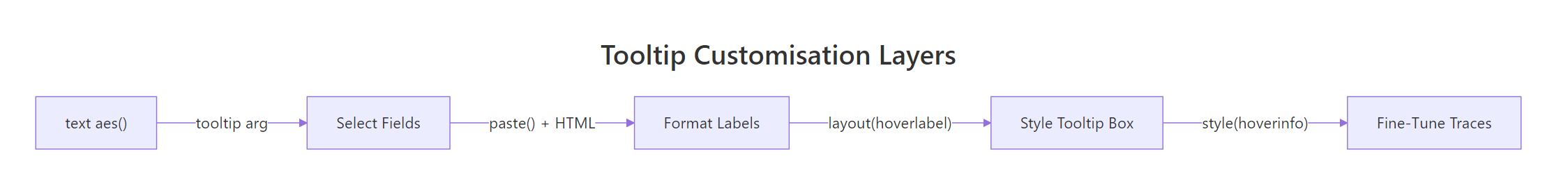
Four layers of tooltip customisation

Figure 2: Four layers of tooltip customisation, from basic text aesthetic to trace-level styling.

For charts with multiple traces — like a line chart with several groups — the default "closest" hover mode shows the tooltip for whichever point is nearest to the cursor. That works for scatter plots, but for time series you often want to compare all y-values at the same x.

economics_long <- tidyr::pivot_longer(economics, cols = c(unemploy, pop), names_to = "metric", values_to = "value") p6 <- ggplot(economics_long, aes(x = date, y = value, color = metric)) + geom_line() + labs(x = "Date", y = "Value") ggplotly(p6) |> layout(hovermode = "x unified") #> One tooltip appears per x-position showing both unemploy and pop values #> Makes it easy to compare the two metrics at any date

Key Insight

"x unified" hover mode is the single biggest readability upgrade for multi-line charts. Instead of chasing individual points, readers see all values at the same x in one tooltip. Set hovermode = "x unified" for any chart with two or more overlapping traces.

Try it: Take the scatter plot from the first section (engine size vs highway MPG) and style the tooltip with a light yellow background ("#FFFFF0") and a font size of 14.

# Try it: style the tooltip box ex_style <- ggplot(mpg, aes(x = displ, y = hwy, color = class)) + geom_point(size = 2) # Add layout(hoverlabel = ...) to ggplotly(): # your code here

Click to reveal solution

ex_style <- ggplot(mpg, aes(x = displ, y = hwy, color = class)) + geom_point(size = 2) ggplotly(ex_style) |> layout(hoverlabel = list( bgcolor = "#FFFFF0", font = list(size = 14) )) #> Tooltip now has light yellow background and larger 14px font

Explanation: layout(hoverlabel = list(...)) accepts bgcolor for background colour and font for text styling. Both apply to every trace.

Which ggplot2 Geoms Translate Well to plotly?

Not every geom survives the conversion equally. Most common geoms — points, lines, bars, boxplots — translate perfectly. A few lose features or need manual adjustment. Knowing which is which saves you debugging time.

Here's a quick demo. All three geoms below convert cleanly.

p_point <- ggplot(mtcars, aes(x = wt, y = mpg)) + geom_point() p_line <- ggplot(economics, aes(x = date, y = unemploy)) + geom_line() p_bar <- ggplot(mpg, aes(x = class)) + geom_bar() ggplotly(p_point) #> Scatter plot — hover shows wt and mpg for each car ggplotly(p_line) #> Line chart — hover shows date and unemployment count ggplotly(p_bar) #> Bar chart — hover shows class and count

All three behave exactly as you'd expect. Now let's look at a geom that needs a small fix: geom_smooth().

p_smooth <- ggplot(mtcars, aes(x = wt, y = mpg)) + geom_point() + geom_smooth(method = "lm", se = TRUE) ggplotly(p_smooth) |> style(hoverinfo = "skip", traces = c(2, 3)) #> The smooth line and CI band no longer produce hover tooltips #> Only the scatter points show tooltips

Without the style() fix, hovering over the confidence band shows unhelpful "upper" and "lower" traces. The style(hoverinfo = "skip", traces = c(2, 3)) call tells plotly to skip hover on the smooth line and its CI band (traces 2 and 3), so only the scatter points respond to hover.

Geom compatibility with ggplotly()

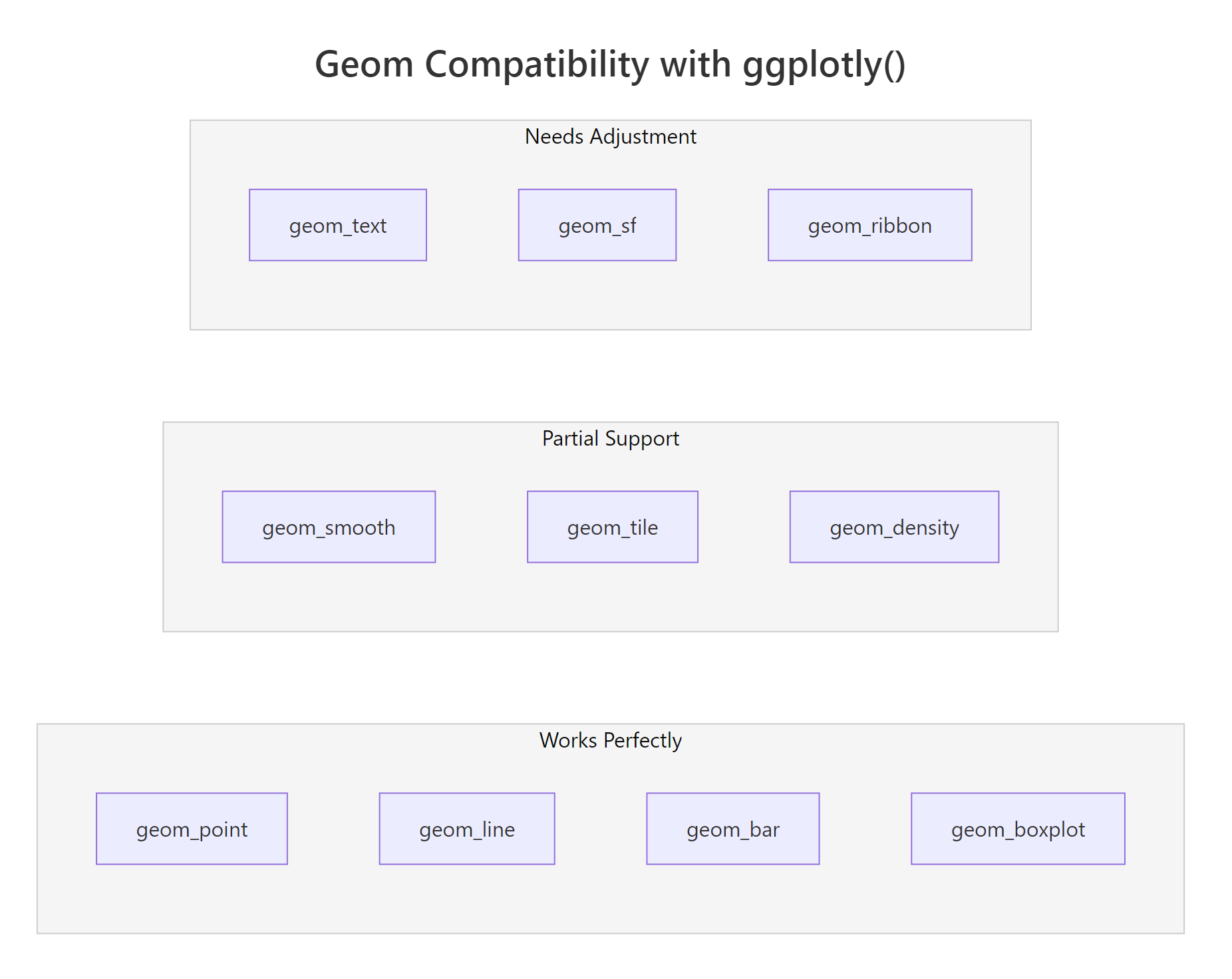
Figure 3: Geom compatibility spectrum — which ggplot2 geoms work best with ggplotly().

Here's the full compatibility table:

Geom	Status	Notes
`geom_point()`	Perfect	All aesthetics carry over
`geom_line()`	Perfect	Hover shows x and y at each point
`geom_bar()` / `geom_col()`	Perfect	Hover shows category and count/value
`geom_boxplot()`	Perfect	Hover shows quartiles, median, outliers
`geom_histogram()`	Perfect	Hover shows bin range and count
`geom_smooth()`	Partial	CI band creates extra hover traces — use `style()` to suppress
`geom_tile()`	Partial	Works, but large heatmaps can be slow
`geom_density()`	Partial	Hover shows density values — sometimes noisy
`geom_text()`	Needs tweaks	Labels may overlap differently — use plotly's `textposition`
`geom_ribbon()`	Needs tweaks	Splits into upper/lower traces
`geom_sf()`	Needs tweaks	Consider plotly's native `plot_geo()` for maps

Warning

Large geom_tile() heatmaps (1000+ cells) can freeze the browser. plotly renders every cell as a separate SVG element. For heatmaps over ~500 cells, use plotly's native plot_ly(type = "heatmap") instead of converting a ggplot2 tile grid.

Let's also look at geom_text(). The labels convert, but plotly sometimes positions them differently than ggplot2.

top_cars <- head(mtcars[order(-mtcars$mpg), ], 5) top_cars$name <- rownames(top_cars) p_text <- ggplot(top_cars, aes(x = wt, y = mpg, label = name)) + geom_point(color = "steelblue", size = 3) + geom_text(nudge_y = 0.8, size = 3.5) ggplotly(p_text) #> Labels appear but may overlap differently than in the static ggplot2 #> Use plotly's layout(annotations = ...) for precise label control

For precise label positioning after conversion, plotly's layout(annotations = ...) gives you pixel-level control. But for most use cases, geom_text() plus a nudge_y works well enough.

Try it: Create a scatter plot of mtcars (wt vs mpg) with a geom_smooth(method = "lm") layer. Convert it with ggplotly() and suppress hover on the smooth trace using style().

# Try it: suppress smooth line hover ex_smooth <- ggplot(mtcars, aes(x = wt, y = mpg)) + geom_point() + geom_smooth(method = "lm") # Convert and use style(hoverinfo = "skip", traces = ...): # your code here

Click to reveal solution

ex_smooth <- ggplot(mtcars, aes(x = wt, y = mpg)) + geom_point() + geom_smooth(method = "lm") ggplotly(ex_smooth) |> style(hoverinfo = "skip", traces = c(2, 3)) #> Only scatter points show hover — smooth line and CI band are silent

Explanation: geom_smooth() creates two extra traces (the fitted line and the confidence band). style(hoverinfo = "skip", traces = c(2, 3)) disables hover on those traces.

How Do You Control Zoom, Pan, and the Toolbar?

By default, click-drag zooms into a rectangular region. Double-click resets. The toolbar (modebar) in the top-right corner offers zoom, pan, lasso select, and download buttons. You can change all of these defaults.

Let's switch the default drag mode from zoom to pan.

p_pan <- ggplot(economics, aes(x = date, y = unemploy)) + geom_line(color = "steelblue") + labs(x = "Date", y = "Unemployed (thousands)") ggplotly(p_pan) |> layout(dragmode = "pan") #> Click-drag now pans the chart instead of zooming #> Useful for long time series where readers want to scroll through time

Panning is more intuitive than zooming for time series, where readers want to scroll left and right through time.

The config() function controls the toolbar buttons. You can remove buttons you don't need, add a custom download format, or hide the toolbar entirely.

ggplotly(p_pan) |> layout(dragmode = "zoom") |> config( displayModeBar = TRUE, modeBarButtonsToRemove = c("select2d", "lasso2d", "autoScale2d"), toImageButtonOptions = list(format = "svg", filename = "my_chart", scale = 2) ) #> Toolbar shows only zoom, pan, reset, and download buttons #> Download button saves a 2x resolution SVG named "my_chart.svg"

For time series data, the range slider gives readers a mini-map at the bottom of the chart. They can drag handles to zoom the x-axis while keeping the global view visible.

p_slider <- ggplot(economics, aes(x = date, y = unemploy)) + geom_line(color = "steelblue") + labs(x = "Date", y = "Unemployed (thousands)") ggplotly(p_slider) |> rangeslider() #> A mini-map appears below the chart #> Drag the handles to zoom into any time range #> The main chart updates in real time

Tip

Add config(toImageButtonOptions = list(format = "svg", filename = "my_chart")) to let users download publication-quality SVGs. The default download format is PNG at screen resolution. SVG scales to any size and is preferred for papers and presentations.

Try it: Take any line chart and set the default drag mode to "select" and remove the "lasso2d" button from the toolbar.

# Try it: customise toolbar ex_toolbar <- ggplot(economics, aes(x = date, y = pop)) + geom_line() # Add layout(dragmode = ...) and config(modeBarButtonsToRemove = ...): # your code here

Click to reveal solution

ex_toolbar <- ggplot(economics, aes(x = date, y = pop)) + geom_line() ggplotly(ex_toolbar) |> layout(dragmode = "select") |> config(modeBarButtonsToRemove = c("lasso2d")) #> Drag mode defaults to box select; lasso button removed from toolbar

Explanation: layout(dragmode = "select") sets the default interaction. config(modeBarButtonsToRemove = ...) removes specific toolbar buttons.

How Do You Animate a ggplot2 Chart with plotly?

plotly can animate your ggplot2 charts — scatter points that move across frames, bars that grow and shrink, lines that evolve. You add a frame aesthetic in ggplot2, and ggplotly() turns it into a play/pause animation with a slider.

Let's create some sample data with three time periods and animate a scatter plot.

set.seed(2026) anim_data <- data.frame( x = rep(1:10, 3), y = c(rnorm(10, 5, 2), rnorm(10, 8, 2), rnorm(10, 12, 2)), group = rep(c("A", "B", "C"), each = 10), year = rep(c(2020, 2022, 2024), each = 10) ) p_anim <- ggplot(anim_data, aes(x = x, y = y, color = group, frame = year)) + geom_point(size = 3) + labs(title = "Animated Scatter by Year", x = "X", y = "Y") ggplotly(p_anim) #> A play button and year slider appear below the chart #> Click play to watch points shift between 2020, 2022, and 2024 #> Each frame shows all three groups at that year

The frame aesthetic tells plotly which variable defines the animation steps. plotly automatically adds a play button and a frame slider. Each unique value of year becomes one frame.

You can fine-tune the animation speed and transition style with animation_opts().

ggplotly(p_anim) |> animation_opts(frame = 800, transition = 400, easing = "elastic") #> Frames last 800ms each, transitions take 400ms with elastic easing #> The animation feels bouncier and more playful

The frame parameter controls how long each frame stays visible (milliseconds). transition controls how long the morph between frames takes. easing accepts CSS easing names like "linear", "elastic", "bounce", and "cubic-in-out".

Key Insight

Animation works by mapping a discrete variable to frame inside aes(). plotly handles the play button, slider, and transitions automatically. You don't need gganimate or any extra package — just one aesthetic mapping.

Try it: Create an animated bar chart that shows the mean mpg for each cyl group in mtcars, using cyl as the frame variable. Use stat_summary() with fun = mean.

# Try it: animated bar chart ex_anim <- ggplot(mtcars, aes(x = factor(gear), y = mpg, frame = factor(cyl))) + # your code here — use stat_summary or geom_col labs(x = "Gears", y = "Mean MPG") # Convert to animated plotly: # your code here

Click to reveal solution

ex_anim <- ggplot(mtcars, aes(x = factor(gear), y = mpg, frame = factor(cyl))) + stat_summary(fun = mean, geom = "col", fill = "steelblue") + labs(x = "Gears", y = "Mean MPG") ggplotly(ex_anim) #> Slider steps through cyl = 4, 6, 8 #> Each frame shows mean MPG per gear for that cylinder count

Explanation: frame = factor(cyl) creates one animation frame per cylinder count. stat_summary() computes the mean for each gear group within each frame.

How Do You Save and Share an Interactive Chart?

Interactive charts aren't PNGs — they're HTML with embedded JavaScript. Saving and sharing them works differently than static plots.

The htmlwidgets::saveWidget() function saves any plotly chart as a self-contained HTML file that anyone can open in a browser.

final_save <- ggplot(mpg, aes(x = displ, y = hwy, color = class)) + geom_point(size = 2) widget <- ggplotly(final_save) htmlwidgets::saveWidget(widget, "my_interactive_chart.html", selfcontained = TRUE) #> File saved: my_interactive_chart.html #> Open in any browser — no R or server needed #> File size: ~3 MB (plotly.js is bundled inside)

The selfcontained = TRUE option bundles the plotly.js library inside the HTML file. The result is a single file anyone can open, even without R installed. The tradeoff is file size — plotly.js adds about 3 MB.

Note

Self-contained HTML files can be 2-5 MB because they bundle plotly.js. For websites and dashboards, use selfcontained = FALSE and host plotly.js separately. For email attachments and one-off sharing, self-contained is simpler.

For R Markdown and Quarto documents, you don't need saveWidget() at all. Just print the plotly object in a code chunk and it renders inline.

Try it: Save one of the previous scatter plots as an HTML file named "scatter_interactive.html".

# Try it: save as HTML ex_save <- ggplot(mtcars, aes(x = wt, y = mpg)) + geom_point() ex_widget <- ggplotly(ex_save) # Save with htmlwidgets::saveWidget(): # your code here

Click to reveal solution

ex_save <- ggplot(mtcars, aes(x = wt, y = mpg)) + geom_point() ex_widget <- ggplotly(ex_save) htmlwidgets::saveWidget(ex_widget, "scatter_interactive.html", selfcontained = TRUE) #> Saved scatter_interactive.html — open in any browser

Explanation: saveWidget() takes a plotly object and writes a standalone HTML file. selfcontained = TRUE bundles everything into one file.

Practice Exercises

Exercise 1: Custom Tooltip Scatter Plot

Build a scatter plot of mtcars with wt on x, mpg on y, coloured by factor(cyl). Create a custom tooltip showing the car name (use rownames(mtcars)), horsepower, and quarter-mile time. Style the tooltip with a white background and 12px font.

# Exercise 1: Custom tooltip + styled hover # Hint: add a name column with rownames(), map text in aes(), use layout(hoverlabel) # Write your code below:

Click to reveal solution

my_cars <- mtcars my_cars$name <- rownames(mtcars) my_p1 <- ggplot(my_cars, aes(x = wt, y = mpg, color = factor(cyl), text = paste0("", name, "", " HP: ", hp, " 1/4 mile: ", qsec, "s"))) + geom_point(size = 3) + labs(x = "Weight (1000 lbs)", y = "MPG", color = "Cylinders") ggplotly(my_p1, tooltip = "text") |> layout(hoverlabel = list( bgcolor = "white", font = list(size = 12) )) #> Hover shows car name (bold), horsepower, and quarter-mile time #> Tooltip has white background with 12px font

Explanation: rownames() provides car names. The text aesthetic with paste0() and HTML tags creates a formatted tooltip. layout(hoverlabel) styles the box.

Exercise 2: Faceted Interactive Chart with Unified Hover

Create a faceted ggplot2 line chart: for each cyl value in mtcars, plot mpg against wt (sorted by wt) using geom_line() + geom_point(). Use facet_wrap(~cyl). Convert to plotly, set hover mode to "x unified", and remove the lasso button from the toolbar.

# Exercise 2: faceted chart + unified hover + toolbar config # Hint: facet_wrap(~cyl), then chain layout() and config() after ggplotly() # Write your code below:

Click to reveal solution

my_sorted <- mtcars[order(mtcars$wt), ] my_sorted$cyl_f <- factor(my_sorted$cyl) my_p2 <- ggplot(my_sorted, aes(x = wt, y = mpg)) + geom_line(color = "steelblue") + geom_point(color = "steelblue", size = 2) + facet_wrap(~cyl_f, scales = "free") + labs(x = "Weight (1000 lbs)", y = "MPG") ggplotly(my_p2) |> layout(hovermode = "x unified") |> config(modeBarButtonsToRemove = c("lasso2d")) #> Three facet panels, each showing mpg vs wt for 4, 6, or 8 cylinders #> Unified hover shows mpg at each weight within a panel #> No lasso button in toolbar

Explanation: facet_wrap() splits the chart. hovermode = "x unified" shows all y-values at a given x. config() removes the lasso tool.

Exercise 3: Animated Scatter with Custom Tooltips

Create a dataset with 3 groups ("Low", "Mid", "High"), 3 years (2020, 2022, 2024), and 8 observations per group-year. Animate a scatter plot by year with custom tooltips showing the group, x value, and y value. Set the transition to 500ms with "cubic-in-out" easing.

# Exercise 3: animated scatter with tooltips # Hint: set.seed(), expand.grid() or manual data.frame, map frame in aes() # Write your code below:

Click to reveal solution

set.seed(99) my_anim_data <- data.frame( x = rep(1:8, 9), y = rnorm(72, mean = rep(c(5, 10, 15), each = 24), sd = 2), group = rep(rep(c("Low", "Mid", "High"), each = 8), 3), year = rep(c(2020, 2022, 2024), each = 24) ) my_p3 <- ggplot(my_anim_data, aes(x = x, y = y, color = group, frame = year, text = paste0("Group: ", group, " X: ", x, " Y: ", round(y, 1)))) + geom_point(size = 3) + labs(x = "X", y = "Y") ggplotly(my_p3, tooltip = "text") |> animation_opts(frame = 800, transition = 500, easing = "cubic-in-out") #> Play button steps through 2020, 2022, 2024 #> Each point shows group, x, and rounded y on hover #> Smooth cubic transitions between frames

Explanation: frame = year creates animation steps. text aesthetic with tooltip = "text" provides custom hover labels. animation_opts() controls timing and easing.

Putting It All Together

Let's build a complete interactive chart from scratch — styled, labelled, and ready to share.

mpg_styled <- mpg mpg_styled$tooltip_text <- paste0( "", mpg_styled$manufacturer, " ", mpg_styled$model, "", " Class: ", mpg_styled$class, " Engine: ", mpg_styled$displ, "L, ", mpg_styled$cyl, " cyl", " Highway: ", mpg_styled$hwy, " mpg", " City: ", mpg_styled$cty, " mpg", " Year: ", mpg_styled$year ) final_p <- ggplot(mpg_styled, aes(x = displ, y = hwy, color = class, size = cty, text = tooltip_text)) + geom_point(alpha = 0.7) + scale_size_continuous(range = c(2, 6), guide = "none") + labs(title = "Fuel Economy by Engine Size", x = "Displacement (L)", y = "Highway MPG", color = "Vehicle Class") + theme_minimal() final_interactive <- ggplotly(final_p, tooltip = "text") |> layout( hoverlabel = list( bgcolor = "white", font = list(family = "Arial", size = 12, color = "#333"), bordercolor = "#ccc" ), hovermode = "closest", dragmode = "zoom" ) |> config( displayModeBar = TRUE, modeBarButtonsToRemove = c("select2d", "lasso2d"), toImageButtonOptions = list(format = "svg", filename = "fuel_economy", scale = 2) ) final_interactive #> Interactive scatter plot with: #> - 234 points sized by city MPG, coloured by class #> - Rich HTML tooltips with model, engine, and mileage details #> - White tooltip box with clean typography #> - Zoom by default, pan available in toolbar #> - SVG download at 2x resolution

This chart combines every technique from the tutorial: custom tooltips with HTML formatting, styled hover labels, curated toolbar buttons, and a meaningful size aesthetic. The reader can explore 234 data points, compare vehicle classes, and download a publication-ready SVG — all from one ggplot2 object wrapped in ggplotly().

Summary

Task	Function / Argument
Convert ggplot2 to interactive	`ggplotly(p)`
Limit tooltip fields	`ggplotly(p, tooltip = c("x", "y"))`
Fully custom tooltip	`aes(text = paste(...))` + `tooltip = "text"`
HTML-formatted tooltip	Use `<b>`, `<br>`, `<i>` inside `paste0()`
Style tooltip box	`layout(hoverlabel = list(bgcolor, font, bordercolor))`
Compare values at same x	`layout(hovermode = "x unified")`
Change drag behaviour	`layout(dragmode = "zoom" / "pan" / "select")`
Customise toolbar	`config(modeBarButtonsToRemove = c(...))`
SVG download button	`config(toImageButtonOptions = list(format = "svg"))`
Range slider (time series)	Pipe to `rangeslider()`
Animate by variable	`aes(frame = var)` in ggplot2
Animation timing	`animation_opts(frame, transition, easing)`
Suppress hover on traces	`style(hoverinfo = "skip", traces = c(...))`
Save as HTML	`htmlwidgets::saveWidget(widget, "file.html")`

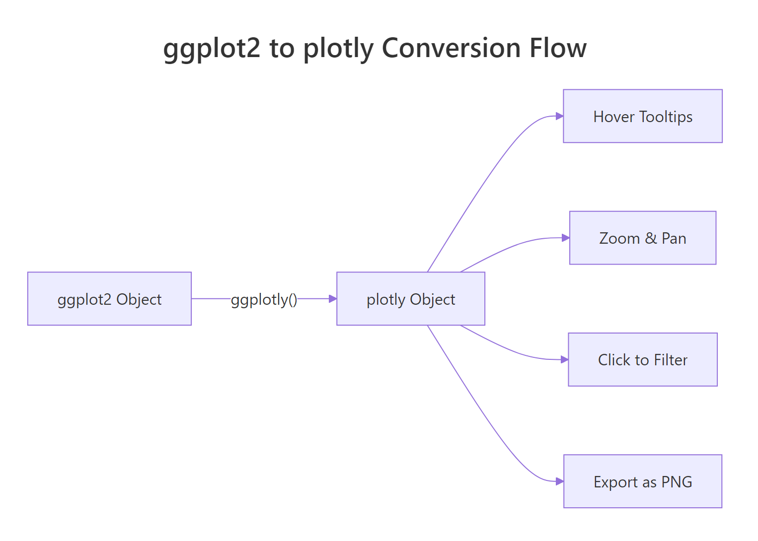
How ggplotly() converts a ggplot2 object into an interactive plotly widget

Figure 1: How ggplotly() converts a ggplot2 object into an interactive plotly widget.

The pattern is always the same: build your chart with ggplot2, wrap it in ggplotly(), then chain layout(), config(), and style() to fine-tune the interactive behaviour. Start with the one-liner, then add layers of customisation as needed.

References

Sievert, C. — Interactive Web-Based Data Visualization with R, plotly, and shiny. CRC Press (2020). Chapters 25 and 33. Link
plotly for R documentation — ggplotly() reference. Link
plotly-r.com — Controlling tooltips. Link
plotly-r.com — Improving ggplotly(). Link
Wickham, H. — ggplot2: Elegant Graphics for Data Analysis, 3rd Edition. Springer (2024). Link
htmlwidgets for R — saveWidget() reference. Link
R Graph Gallery — Customize plotly tooltip. Link

Continue Learning

ggplot2 Getting Started — Build your first 5 charts with ggplot2 before making them interactive
ggplot2 Themes in R — Polish your static charts with themes, then convert to plotly
ggplot2 Scatter Plots — Deep dive into scatter plot customisation — all techniques carry over to plotly

r‑statistics.co by Selva Prabhakaran

ggplot2 + plotly: Add Hover Tooltips and Zoom to Any Chart in One Line

How Does ggplotly() Turn a Static Chart Interactive?

How Do You Control What Appears in the Tooltip?

How Do You Style the Tooltip Box Itself?

Which ggplot2 Geoms Translate Well to plotly?

How Do You Control Zoom, Pan, and the Toolbar?

How Do You Animate a ggplot2 Chart with plotly?

How Do You Save and Share an Interactive Chart?

Practice Exercises

Exercise 1: Custom Tooltip Scatter Plot

Exercise 2: Faceted Interactive Chart with Unified Hover

Exercise 3: Animated Scatter with Custom Tooltips

Putting It All Together

Summary

References

Continue Learning

On this page

r‑statistics.co by Selva Prabhakaran

ggplot2 + plotly: Add Hover Tooltips and Zoom to Any Chart in One Line

How Does ggplotly() Turn a Static Chart Interactive?

How Do You Control What Appears in the Tooltip?

How Do You Style the Tooltip Box Itself?

Which ggplot2 Geoms Translate Well to plotly?

How Do You Control Zoom, Pan, and the Toolbar?

How Do You Animate a ggplot2 Chart with plotly?

How Do You Save and Share an Interactive Chart?

Practice Exercises

Exercise 1: Custom Tooltip Scatter Plot

Exercise 2: Faceted Interactive Chart with Unified Hover

Exercise 3: Animated Scatter with Custom Tooltips

Putting It All Together

Summary

References

Continue Learning

Related Tutorials

On this page