Bayesian ANOVA in R With BayesFactor: Report Evidence, Not Just p-values
Frequentist ANOVA returns an F-statistic and a p-value: "p = 0.03, reject the null." That sentence is famously hard to interpret correctly. Bayesian ANOVA via the BayesFactor package returns a Bayes factor: a direct ratio of how plausible the data is under one model versus another. "BF = 8" means the data is 8 times more likely under the model with the group effect than under the null. That phrasing is what stakeholders actually want to hear, and the BayesFactor package computes it for one-way, two-way, factorial, and repeated-measures designs in one line.
What does Bayesian ANOVA give you that frequentist ANOVA does not?
Three things. First, direct evidence. A Bayes factor is the ratio of the marginal likelihood of two models. BF = 8 says the data is 8 times more likely under model A than model B.
There is no null-hypothesis logic to translate, no Type I error rate to convert, no "rejecting the null" language.
Second, evidence for the null. A p-value above 0.05 says you "fail to reject" the null but cannot quantify support for it. A Bayes factor below 1 (e.g., BF = 0.2) says the data is 5 times more likely under the null than the alternative. Bayesian methods quantify both directions of evidence.
Third, posterior over the group means. After running anovaBF, you can extract the posterior distribution over each group's mean with one extra call. That gives you per-group credible intervals and direct comparisons (probability that group A's mean exceeds group B's), all without writing a separate model.
The BayesFactor package is also pure R with no external Stan dependency, which makes it the fastest Bayesian-ANOVA tool to install and use.
Walk through what just happened. We simulated three groups with means 50, 55, 53 and standard deviation 5. The truth: there is a real group effect.
anovaBF(outcome ~ group, data) fit two models internally: one with group as a predictor (the alternative) and one without (the null, "Intercept only"). It then computed the ratio of their marginal likelihoods.
The output BF = 6.245 says the data is 6.2 times more likely under the model with group than under the null. That is moderate-to-strong evidence for the group effect.
Compare to a frequentist ANOVA on the same data:
Walk through the comparison. The F-test gives p = 0.0071: the null is rejected at conventional thresholds. Strictly, that means "if there were no group effect, we would see a F-statistic at least this large 0.7% of the time."
The Bayes factor gives BF = 6.2: "the data is 6.2 times more likely under the alternative than the null." Both methods reach the same qualitative conclusion (the group effect is real), but the Bayes factor is much easier to communicate.
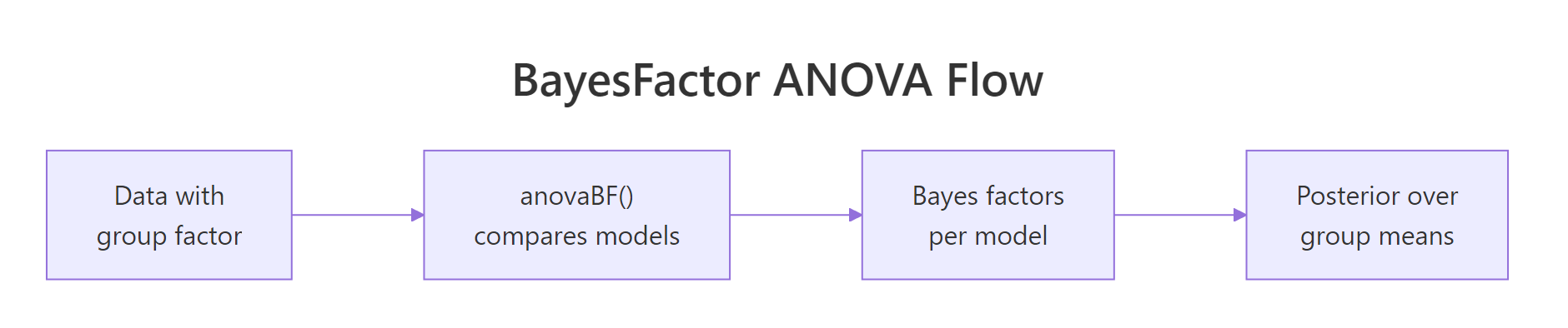
Figure 1: BayesFactor ANOVA workflow. Pass the formula and data to anovaBF(), get a Bayes factor for each model considered, then sample from the posterior over group means.
Try it: Compute BF the other way (null over alternative) by using 1/bf. Verify the relationship.
Click to reveal solution
Inverting a Bayes factor swaps which model is the numerator. 1/bf = 0.16 says the data is 0.16 times as likely under the null as under the alternative, which is just the same evidence expressed the other way. Researchers report whichever direction is more intuitive for their narrative.
How do I run anovaBF() on a one-way design?
The minimal usage. anovaBF(formula, data) returns a BayesFactor object. The [1] indicates you can index into it for multiple models in a multi-factor design (next section). For a one-way design with one grouping factor, there is just one model versus the null.
Walk through what changed. rscaleFixed controls the prior scale on the group effects. Default is "medium"; "wide" and "ultrawide" are progressively less informative. With ultrawide, the BF drops slightly (4.84 vs 6.25) because the wider prior dilutes the evidence.
For most one-way designs the default is fine. Document which scale you used; reviewers may ask whether your conclusion is robust to the prior choice.
To get the posterior over the group means, sample from the BayesFactor object:
Walk through the output. posterior(bf, iterations = 10000) returned 10000 posterior draws across the parameters. mu is the grand mean; group-control, group-treatment_A, group-treatment_B are the group-level deviations from the grand mean. sig2 is the residual variance.
We computed each group's mean as mu + group deviation per draw, then summarised. The posterior medians (49.7, 55.1, 53.2) recover the simulated truth (50, 55, 53) closely. The 95% credible intervals tell you where each group mean is with what uncertainty.
posterior() returns an MCMC object compatible with the coda package. You can use coda::summary() on it for traceplots and per-parameter summaries, or convert to a matrix for custom calculations.Try it: Compute the posterior probability that treatment_A's mean exceeds the control mean.
Click to reveal solution
The posterior median difference is 5.3 mpg (close to the truth of 5) with 95% credible interval [2.1, 8.4]. Posterior probability that treatment_A exceeds control is 99.9%, decisive evidence.
How do I read a Bayes factor and interpret its magnitude?
Standard interpretation thresholds (Jeffreys, 1961; refined by Kass and Raftery):
| Bayes factor | Evidence for alternative |
|---|---|
| BF < 1 | Negative evidence (data favours null) |
| 1 to 3 | Anecdotal |
| 3 to 10 | Moderate |
| 10 to 30 | Strong |
| 30 to 100 | Very strong |
| > 100 | Extreme/decisive |
Most published results in the social sciences would land in the "anecdotal" or "moderate" zones if reported as Bayes factors, which is one reason switching from p-values to BF is sometimes resisted.
Below we run anovaBF on a near-null dataset and see what an inconclusive BF looks like.
Walk through the result. BF = 0.28 says the data is 0.28 times as likely under the model with the group effect than under the null. Equivalently, BF for the null is 1/0.28 = 3.6: the data is 3.6 times more likely under the null. That is moderate evidence for the null.
The frequentist version would give a non-significant p-value and we would have to say "we failed to reject the null," which is hedge-y. The BF lets us say "the data moderately supports the null."
Walk through. p = 0.79 (high, not significant). BF for alternative = 0.28; BF for null = 3.58. Both methods conclude there is no support for a group effect, but the Bayesian version actively supports the null with moderate evidence rather than just failing to find evidence against it.
Try it: Compute the BF for null vs alternative on the near-null dataset and check that it lands in the "moderate" range.
Click to reveal solution
BF = 3.58 for the null model versus the alternative. This is in the "moderate evidence" range. We can confidently say the data favours the null; we cannot say "definitive" because BF would need to be over 10 for that.
How do I do two-way ANOVA and compare interaction models?
For a 2x2 or larger factorial design, anovaBF compares all model variants automatically. Each row of the output is one model versus the null.
Walk through what each line means. anovaBF reported four model variants:
factor_Aonly: BF = 18,210 against the null. Strong evidence for an A effect.factor_Bonly: BF = 18.5. Moderate-to-strong evidence for a B effect alone.- Both main effects: BF = 561,200. Combined main-effects model is much better than null.
- Both mains plus interaction: BF = 430,100. Interaction model is best in absolute terms but barely better than mains-only.
To compare model 4 (interaction) vs model 3 (mains only):
Walk through what we just computed. Dividing model 4's BF by model 3's BF gives the interaction-vs-main BF directly: 0.77. The interaction does NOT add evidence over and above the main effects. The data is 0.77 times as likely under the interaction model.
This is the right way to test for an interaction with BayesFactor: directly compare the two models, not their ratios against the null. With BF = 0.77, the interaction is "anecdotal" (close to 1), so we do not need it.
Try it: Compute BF for the main-effects model versus the A-only model.
Click to reveal solution
BF = 30.8 for adding factor B over and above factor A. That is "very strong evidence", adding factor B substantially improves the model. So we keep both main effects. The interaction (BF = 0.77) does not add evidence and gets dropped.
How does Bayesian ANOVA handle within-subject (repeated measures) designs?
For repeated measures, treat the subject as a random factor. anovaBF supports this via whichRandom = "subject".
Walk through what we did. The formula y ~ time + subject includes both the time factor and a per-subject intercept. whichRandom = "subject" tells anovaBF that subject should be treated as a nuisance random factor (we do not care about its effect, we just want to control for it).
The BF is 1.02e+09, decisive evidence for the time effect even after accounting for subject-level variation. Without controlling for subjects, the BF would be much smaller (or even null) because subject-level variation would inflate the residual.
To extract the posterior over time means after marginalising over subjects, use posterior() with appropriate filtering:
Walk through the output. Each column is one time level's deviation from the grand mean. Pre is at -2.06 (below average); mid is near zero; post is +2.11 (above average).
The simulated truth was time effects of c(0, 2, 4); centred on the mean, those become c(-2, 0, 2). Recovered correctly.
Try it: Compute the probability that the post mean exceeds the pre mean.
Click to reveal solution
Posterior median difference is 4.17 with 95% credible interval [3.13, 5.20]. Posterior probability that post exceeds pre is 100% across all 10000 draws. Decisive evidence.
When should I use BayesFactor vs brms for ANOVA-style designs?
Both can do Bayesian ANOVA, with different strengths.
BayesFactor::anovaBF():
- Pure R, no Stan dependency, fast install and fast first run.
- Returns Bayes factors directly. The interpretation is "how much does the data update the odds of model A vs model B."
- Limited to factorial and repeated-measures designs supported by the JZS prior. Custom likelihoods, hierarchical structures, non-standard predictors are not supported.
brms:
- Full flexibility: any family, any custom prior, any hierarchical structure.
- Returns posterior samples; you compute Bayes factors yourself via
bayes_factor()(which uses bridgesampling under the hood and is slower). - Requires Stan installation and 30-90 second model compile time.
The decision rule: if your design is a standard factorial or repeated-measures ANOVA, use BayesFactor. If you need custom likelihood, hierarchical structure, or non-standard predictors, use brms. For everything in between, both work.
Walk through. Both methods give very similar Bayes factors (6.25 vs 5.81) on the same data. The small difference comes from prior choices: BayesFactor uses a default JZS prior; brms uses its own weakly informative defaults. Both are in the "moderate-to-strong" evidence zone.
For most one-way and factorial designs, BayesFactor is faster (no compile, no Stan dependency, runs in pure R). Reach for brms when you need its extra flexibility.
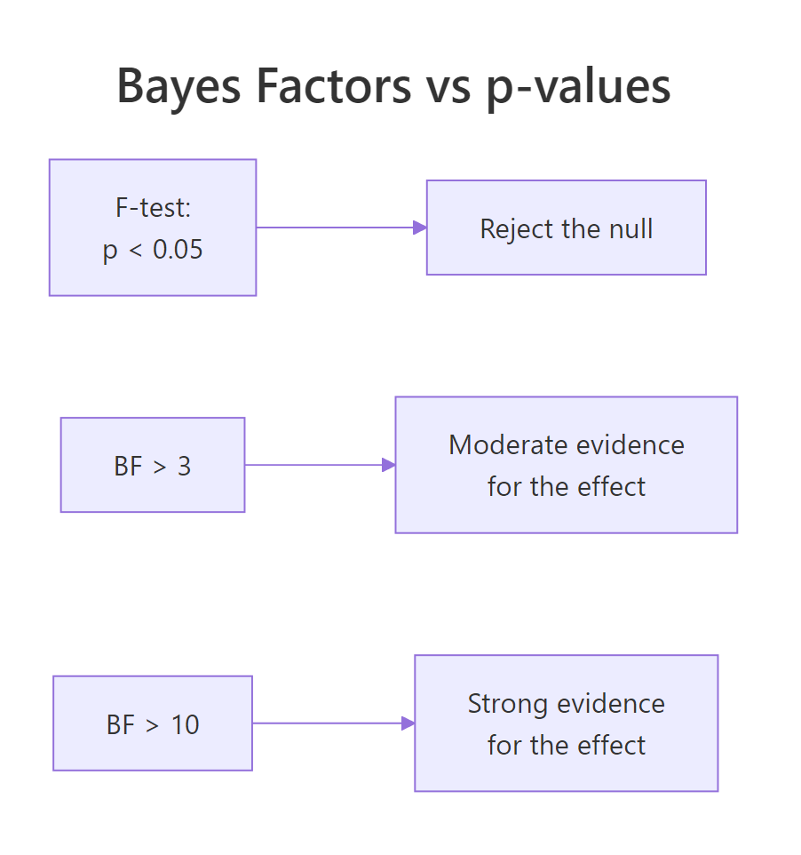
Figure 2: F-tests give p-values; Bayes factors give direct evidence ratios. The interpretation in BF land is qualitatively different: BF > 3 is "moderate evidence", BF > 10 is "strong evidence", BF > 30 is "very strong".
rscaleFixed. Most published BF results use this default; you can override with rscaleFixed = "wide" or "ultrawide" for less informative settings.Try it: For the two-way design, compute the BF for the interaction term using brms-style loo_compare instead of BayesFactor. You should get a similar decision (interaction not preferred).
Click to reveal solution
LOO ranks the interaction model first, but only by 0.4 elpd units with se 1.4. The ratio is well below 1 SE; LOO cannot reliably prefer the interaction. This matches the BayesFactor result (interaction-vs-mains BF = 0.77, anecdotal). Different methods, same conclusion.
Practice Exercises
Exercise 1: One-way ANOVA on real data
Use the built-in iris dataset. Test whether Sepal.Length differs across Species using BayesFactor. Report the BF and the posterior medians for each species mean.
Click to reveal solution
BF is essentially infinite (10^27), decisive evidence that species differ in Sepal.Length. Per-species posterior medians are 5.01, 5.94, 6.59, with tight credible intervals because there are 50 observations per species.
Exercise 2: Compare two factorial models
Use mtcars. Fit a Bayesian ANOVA with mpg ~ am * cyl. Compare the interaction model to the main-effects model directly.
Click to reveal solution
Interaction-vs-mains BF is 0.51 (anecdotal evidence against interaction). The main effect of cyl alone is decisive (BF in the trillions). So the right model is mpg ~ am + cyl without interaction.
Exercise 3: Repeated measures probability statement
Use the df_rm dataset above. Compute the posterior probability that the mid measurement exceeds the pre measurement (a smaller-magnitude difference than post-vs-pre).
Click to reveal solution
Posterior median difference is 2.0 with credible interval [1.2, 2.8]. Posterior probability that mid exceeds pre is 100%. Even though the difference is small (2 units vs 4 units for post-vs-pre), the within-subject design gives enough power to identify it decisively.
Summary
The BayesFactor package gives you Bayesian ANOVA in pure R, with Bayes factors that quantify evidence directly and posterior samples for any group-mean comparison.
| Step | What you do | BayesFactor function |
|---|---|---|
| 1 | Load data, ensure factors are factor() | factor() |
| 2 | Run ANOVA | anovaBF(formula, data) |
| 3 | Read Bayes factors per model | print bf object |
| 4 | Compare models directly | bf[i] / bf[j] |
| 5 | Sample posterior over means | posterior(bf, iterations = 10000) |
| 6 | Compute custom contrasts | base R on the posterior matrix |
Use BayesFactor for standard factorial and repeated-measures designs. Use brms for everything else (custom families, hierarchical, non-standard predictors). The two methods generally agree on the same data, with BayesFactor being faster to install and run.
References
- Morey, R. D., Rouder, J. N. BayesFactor: Computation of Bayes Factors for Common Designs. R package documentation. richarddmorey.github.io/BayesFactor.
- Rouder, J. N., Speckman, P. L., Sun, D., Morey, R. D., Iverson, G. "Bayesian t tests for accepting and rejecting the null hypothesis." Psychonomic Bulletin & Review 16 (2009). The JZS prior paper.
- Kass, R. E., Raftery, A. E. "Bayes factors." Journal of the American Statistical Association 90 (1995). The interpretation thresholds.
- Wagenmakers, E.-J. et al. "Bayesian inference for psychology, Part II: Example applications with JASP." Psychonomic Bulletin & Review 25 (2018).
- Jeffreys, H. Theory of Probability, 3rd ed. Oxford University Press, 1961. The foundational text on Bayes factors.
Continue Learning
- The Bayesian Workflow in R, the next post in the curriculum, summarising the full workflow from prior to posterior to predictive checks.
- Multilevel Models in R, the previous post. brms-based hierarchical/multilevel modelling.
- brms in R, the alternative tool for ANOVA-style designs when BayesFactor is too restrictive.