Write Better R Functions: Arguments, Defaults, Scope & When to Vectorise
An R function is a reusable block of code you define once with function() and call any time. Good R functions take named arguments, provide sensible defaults, return one clear value, and fail loudly on bad input, so you stop copy-pasting the same five lines across your script.
Why wrap code in a function at all?
Because the same five lines copy-pasted four times is four places a bug can hide. A function turns that repetition into a single tested unit you can call with one line. Here's what the payoff looks like, a three-line function that replaces a block you'd otherwise write for every numeric vector.
One definition, infinite reuse. Change the formula in one place and every caller gets the fix. Functions are also the unit you test, document, and share, R has no concept of "reusable code" smaller than a function.
Try it: Write a one-line function ex_celsius_to_f that converts Celsius to Fahrenheit (formula: C * 9/5 + 32) and call it on c(0, 20, 100).
Click to reveal solution
The body is a single expression, so there's no need for return(), the last (and only) expression is returned automatically. The formula is vectorised, so c(0, 20, 100) is converted element-by-element to c(32, 68, 212) in one call.
How do you declare a function and what's in the signature?
Every R function has three parts: a name (how you'll call it), a signature (the arguments it accepts), and a body (the code that runs). You bind all three with function() and save it to a variable.
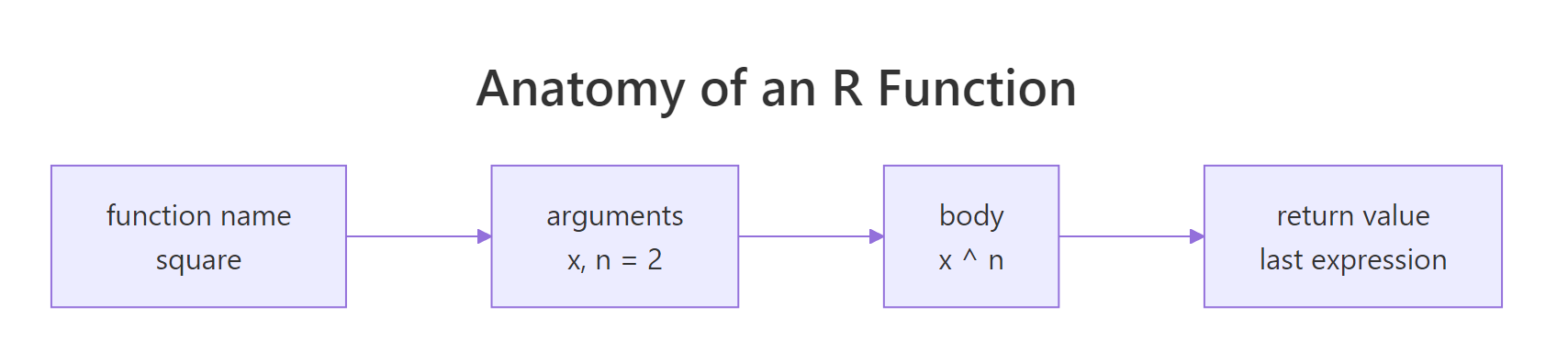
Figure 1: The four pieces of every R function, the name you bind it to, the argument list, the body, and the return value.
Two arguments: x (required, no default) and digits (optional, defaults to 2). The body computes three statistics and returns a rounded named vector. Notice there's no return(), R returns the value of the last expression automatically. We'll come back to that.
summarise_vector is a variable whose value happens to be a function. You can pass it to other functions, store it in a list, or reassign it.Try it: Modify summarise_vector so it also returns the min and max. Call it ex_summarise_v2 and run it on c(4, 7, 9, 12, 15, 18).
Click to reveal solution
Appending min = min(x) and max = max(x) to the named vector extends the return value without changing the rest of the function, the round() call then applies uniformly to all five entries. A named numeric vector is a fine lightweight return when every field is the same type; reach for a list() only when the pieces have different shapes.
How do default arguments and positional/named matching really work?
When you call a function, R matches your arguments in three passes: exact name match first, then partial name match, then positional match. Defaults fill in anything the caller didn't supply. Understanding this order prevents most "why did my function get the wrong value?" bugs.
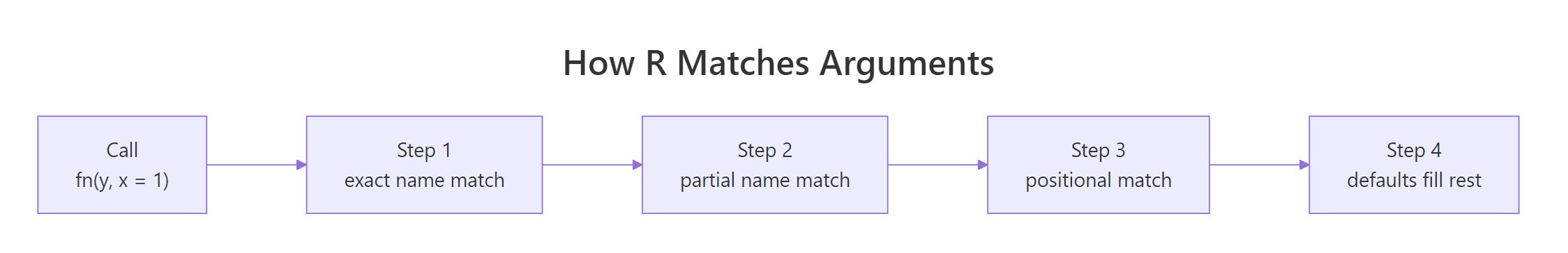
Figure 2: How R matches call-site arguments to a function's formal parameters, exact name wins, then partial, then position.
Named arguments are almost always clearer at the call site. If a reader can't tell what TRUE, FALSE, 3 means without looking up the signature, you should be writing scale = TRUE, center = FALSE, k = 3.
greet(punct = "?") works today; tomorrow someone adds punctuate_words and your call becomes ambiguous. Prefer full names.Try it: Call greet with name = "Lin" and greeting "Hey", using the punctuation default. Save it to ex_msg.
Click to reveal solution
Passing name and greeting by name lets R skip the positional order and leaves punctuation to fall back to its default of "!". Named arguments like this are how you communicate intent to the reader and stay safe if the function author ever reorders the signature.
Should you use return() explicitly or rely on implicit return?
R returns the value of the last expression in the function body automatically. return() exists mainly for early exits, bailing out before the end of the function. For the happy path, leave it off.
Two idioms, one rule: use return() when you want to stop early. Don't sprinkle return() on every final line, it's noise. A function that returns something on every branch without return() reads more clearly than one littered with them.
list(). R has no tuples, lists are how you bundle heterogeneous return values.Try it: Write ex_range_info(x) that returns a list with min, max, and span (max minus min). Test on c(4, 9, 2, 7).
Click to reveal solution
Wrapping the three values in list() lets the single return carry heterogeneous pieces, if you used c() the elements would all collapse to one numeric vector and you'd lose the names' semantic distinction. Callers pull individual fields back out with $min, $max, $span.
How does R find variables inside a function (lexical scoping)?
When a function needs a variable, R first looks inside the function, then in the environment where the function was defined, then up the chain to the global environment, and finally in attached packages. This is lexical scoping, "lexical" because the lookup follows the code's written structure, not its call order.
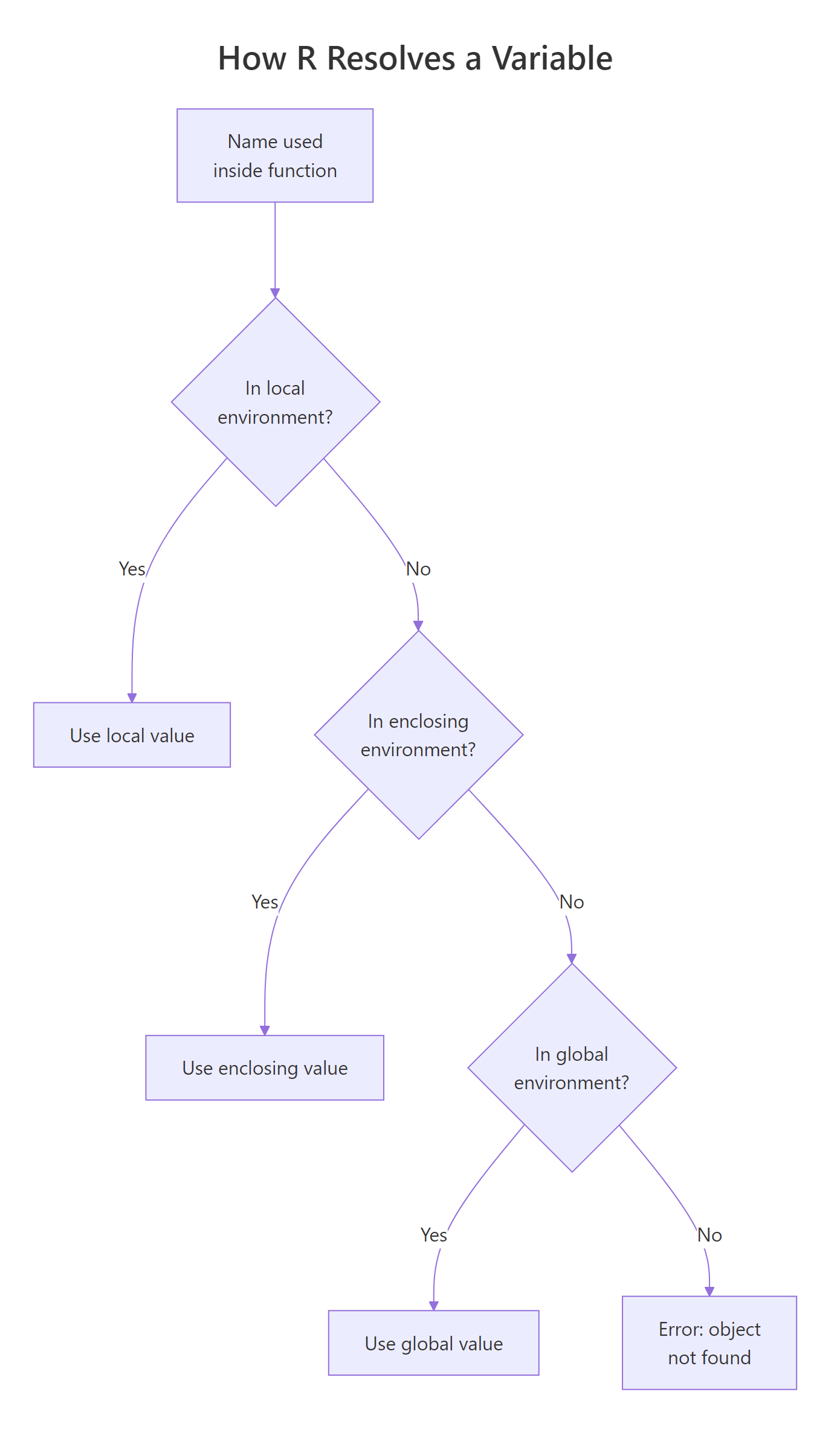
Figure 3: R's scope chain. A name is resolved by walking outward from the function's own environment through each enclosing environment until it's found.
multiplier isn't an argument, but R finds it in the global environment. This "reaching out" is powerful but also a trap, your function's behavior now depends on an invisible variable. Change multiplier elsewhere and scale_up silently changes too.
options()). Pass everything the function needs as arguments. Future-you will thank you.The second half of lexical scoping is that assignments inside a function stay inside, they don't leak out.
Each call to increment() creates its own local counter, uses it, and throws it away. The global counter is untouched. This is R's copy-on-modify model in action, functions can't accidentally corrupt the caller's variables.
Try it: Define ex_g <- 100. Write ex_shift(x) that returns x + ex_g. Call it with x = 5, then set ex_g <- 200 and call again. What do you predict?
Click to reveal solution
ex_shift() has no ex_g in its own environment, so R walks outward and picks up the current value from the global environment at call time, not at definition time. That's why changing ex_g to 200 between the two calls changes the result. It's also why leaning on globals inside functions is fragile: a caller can silently alter the result without touching the arguments.
When should you vectorise vs loop inside a function?
R's built-in operators and most functions are already vectorised, they apply element-wise to whole vectors in a single, fast C call. A for-loop in R is dramatically slower because each iteration pays interpreter overhead. The rule: if a vectorised version exists, use it.
Same answer, one-third the code, and on a million-element vector normalise_vec is roughly 50-100x faster. The vectorised version also reads like the math: subtract the min, divide by the range.
+, -, *, /, ifelse(), pmax(), pmin(), cumsum(), or an apply family function?" Nine times out of ten, yes.Loops aren't forbidden, they're the right tool when each iteration depends on the previous result (like a simulation), or when you're calling a function that isn't itself vectorised. Write the loop then; don't apologise for it.
Try it: Write ex_standardise(x) that returns (x - mean(x)) / sd(x), vectorised, one line. Test on c(1, 2, 3, 4, 5).
Click to reveal solution
mean(x) and sd(x) each collapse the vector to a scalar, and the surrounding arithmetic is recycled across every element of x in a single C call. The result is a vector with mean 0 and standard deviation 1, the same thing scale() does, minus the matrix wrapper.
How do you validate inputs and fail loudly, not silently?
A function that accepts garbage and returns garbage is worse than one that crashes, the silent failure shows up three steps later with no trace of where it started. Validate at the top with stopifnot() or explicit stop() calls, so bad input fails immediately with a clear message.
Each named string in stopifnot() is both the condition's description and the error message shown when it fails. If a caller hands in a character vector, they get Error: x must be numeric instantly, not a cryptic NaN ten functions downstream.
For more structured errors with classes and metadata, see rlang::abort(). For warnings that shouldn't stop execution, use warning(). But 80% of the time, stopifnot() is all you need.
Try it: Write ex_mean_positive(x) that returns mean(x) but uses stopifnot() to require x is numeric and all positive.
Click to reveal solution
The two stopifnot() conditions run before the body, so a character vector or any value <= 0 raises the matching error immediately instead of silently flowing into mean(). Named strings on the left-hand side of each assertion become the error message, make them explicit enough that the caller understands the contract without reading the function body.
Practice Exercises
These capstones combine multiple concepts from the sections above. Aim to write each function from scratch before peeking.
Exercise 1: A reusable summary function
Write describe(x, digits = 3) that returns a named list with n, mean, sd, min, max, and range of a numeric vector. Validate that x is numeric and non-empty. Round numeric results to digits.
Show solution
Exercise 2: Min-max scaler with a fallback
Write scale_minmax(x, fallback = 0) that rescales x to [0, 1]. If all values of x are identical (zero range), return a vector of fallback the same length as x. Use an early return().
Show solution
Exercise 3: A function that returns a function
Write make_power(exp) that returns a new function which raises its input to the power exp. Use it to build square and cube.
Show solution
The inner function "remembers" exp because of lexical scoping, that's a closure.
Complete Example: A Grouped Summary Function
Let's put everything together. We'll write group_stats(df, group_col, value_col), a function that takes a data frame, groups by one column, and returns mean and sd for another. It validates inputs, uses sensible defaults, and has an early return for empty data.
One call, real output. The function is general, swap "cyl" for "gear" and "mpg" for "hp" and it just works. That reusability is the whole point.
Summary
| Concept | Rule of thumb |
|---|---|
| Declare | name <- function(args) { body }, a function is just an object |
| Arguments | Required first, optional (with defaults) after. Prefer named calls. |
| Return | Last expression returns implicitly. Use return() only for early exits. |
| Multiple values | Wrap in list(), R has no tuples. |
| Scoping | Lexical: look local first, then enclosing, then global, then packages. |
| Globals | Don't read them inside functions. Pass everything as arguments. |
| Vectorise | Default to element-wise operators. Loop only when iterations depend on each other. |
| Validate | stopifnot() at the top. Fail fast, fail loud, with clear messages. |
Functions are how you turn scripts into software. Master these seven habits and your R code stops being a pile of snippets and becomes a toolkit.
References
- Wickham, H. Advanced R, 2nd ed., Chapter 6 (Functions).
- R Core Team. An Introduction to R, Section 10: Writing your own functions.
- Wickham, H. & Grolemund, G. R for Data Science, 2nd ed., Chapter 25: Functions.
- R Documentation.
?function,?stopifnot,?match.arg,?missing. Run in any R session. - Morandat, F. et al. Evaluating the Design of the R Language (2012), scoping and semantics.
- Tidyverse style guide, function naming and argument order.
Continue Learning
- Control Flow in R,
if,else,for,while, the building blocks you'll use inside function bodies. - R Vectors, understand the data structures your functions will operate on.
- Functional Programming in R,
map(),reduce(), and treating functions as first-class objects.