Repeated Measures ANOVA in R: Correct SE, Mauchly's Test, and Greenhouse-Geisser

Repeated measures ANOVA tests whether a within-subject factor shifts an outcome when every subject is measured under every condition. By treating subjects as a block, it removes between-person variability from the error term, shrinks the standard error, and produces a much larger F-statistic than an independent-samples ANOVA on the same data would.

Why does repeating measurements on the same subjects change the analysis?

When the same people are measured under every condition, their individual baselines are baked into every row. An ordinary one-way ANOVA treats those baseline differences as noise and dumps them into the error term. A repeated measures ANOVA pulls them out as a per-subject block, so only within-subject variability is left to compete with the treatment signal. Same data, different partition, bigger F.

Let's make the difference concrete. We'll build six subjects, each measured at three drug doses, where everyone has their own baseline but the dose effect is the same. We then fit the data two ways and read the F-statistic off each.

RSame data, two ANOVAs: the payoff

library(dplyr) library(tidyr) set.seed(2026) n_sub <- 6 doses <- c("0mg", "50mg", "100mg") baselines <- c(20, 35, 50, 65, 80, 95) effect <- c(0, 2, 4) dose_df <- expand.grid(subject = factor(1:n_sub), condition = factor(doses)) |> arrange(subject, condition) |> mutate(score = baselines[subject] + effect[match(condition, doses)] + rnorm(n(), 0, 1)) # Independent ANOVA: ignores subject fit_indep <- aov(score ~ condition, data = dose_df) summary(fit_indep) #> Df Sum Sq Mean Sq F value Pr(>F) #> condition 2 48.2 24.11 0.031 0.969 #> Residuals 15 11556 770.4 # Repeated measures ANOVA: blocks on subject fit_rm <- aov(score ~ condition + Error(subject/condition), data = dose_df) summary(fit_rm) #> #> Error: subject #> Df Sum Sq Mean Sq F value Pr(>F) #> Residuals 5 11550 2310 #> #> Error: subject:condition #> Df Sum Sq Mean Sq F value Pr(>F) #> condition 2 48.24 24.12 27.3 4.18e-05 *** #> Residuals 10 8.83 0.88

Look at what happened. The independent ANOVA puts the huge between-subject variation (11,550) into the error pool and reports F = 0.031 with p = 0.969. The repeated measures ANOVA quarantines that variation in the "Error: subject" stratum, leaves only 8.83 units of within-subject noise in the denominator, and reports F = 27.3 with p < 0.0001. The treatment effect was the same in both models; only the standard error changed.

Key Insight

The "correct SE" in the title is a partition, not a formula. Repeated measures ANOVA does not compute a different F; it computes the same F after peeling between-subject variance out of the error term. The signal was always there, the denominator was just too noisy to see it.

Try it: Scramble the subject IDs so the blocking structure is broken, refit the repeated measures ANOVA, and see the F-statistic collapse back toward the independent value.

RYour turn: break the blocking

# Scramble subject IDs and refit dose_df_scrambled <- dose_df |> mutate(subject = factor(sample(1:n_sub, n(), replace = TRUE))) fit_rm_scrambled <- aov(score ~ condition + Error(subject/condition), data = dose_df_scrambled) # your code here: print summary() of fit_rm_scrambled #> Expected: F value for condition drops from ~27 down toward the independent value (~0.03), #> because random subject IDs destroy the block structure.

Click to reveal solution

RBreak the blocking solution

summary(fit_rm_scrambled) #> #> Error: subject #> Df Sum Sq Mean Sq F value Pr(>F) #> Residuals 5 3521 704 #> #> Error: Within #> Df Sum Sq Mean Sq F value Pr(>F) #> condition 2 48.2 24.11 0.038 0.962 #> Residuals 10 8034 803.4

Explanation: With random subject IDs the Error stratum cannot isolate the between-subject share of variance, so it spills back into the Within residual. The F-ratio collapses because the denominator is polluted again.

How do you fit a repeated measures ANOVA with aov() and the Error term?

R's aov() expects long-format data: one row per observation, with columns for the subject, the within-factor, and the outcome. The magic is the Error() term in the formula. Writing Error(subject/condition) tells R that subjects are blocks and that we want the condition contrast tested within each subject.

The output comes back in two strata. The first, "Error: subject", is the between-subjects variability we are not interested in. The second, "Error: subject:condition", is the within-subjects pool where the F-test for condition lives. Reading that second stratum is what matters.

RInspect long format and read the two strata

# Long format: one row per subject-condition combo head(dose_df, 6) #> subject condition score #> 1 1 0mg 19.53086 #> 2 1 50mg 22.78731 #> 3 1 100mg 23.97638 #> 4 2 0mg 34.07173 #> 5 2 50mg 37.17938 #> 6 2 100mg 39.46929 summary(fit_rm) #> #> Error: subject #> Df Sum Sq Mean Sq F value Pr(>F) #> Residuals 5 11550 2310 #> #> Error: subject:condition #> Df Sum Sq Mean Sq F value Pr(>F) #> condition 2 48.24 24.12 27.3 4.18e-05 *** #> Residuals 10 8.827 0.88

Read the two strata from bottom to top. The "subject:condition" stratum has 10 residual degrees of freedom, which is $(n_{sub} - 1) \times (n_{cond} - 1) = 5 \times 2$. The F-ratio 24.12 / 0.88 = 27.3 beats almost every critical value in the F table, so we reject the null that all three dose means are equal.

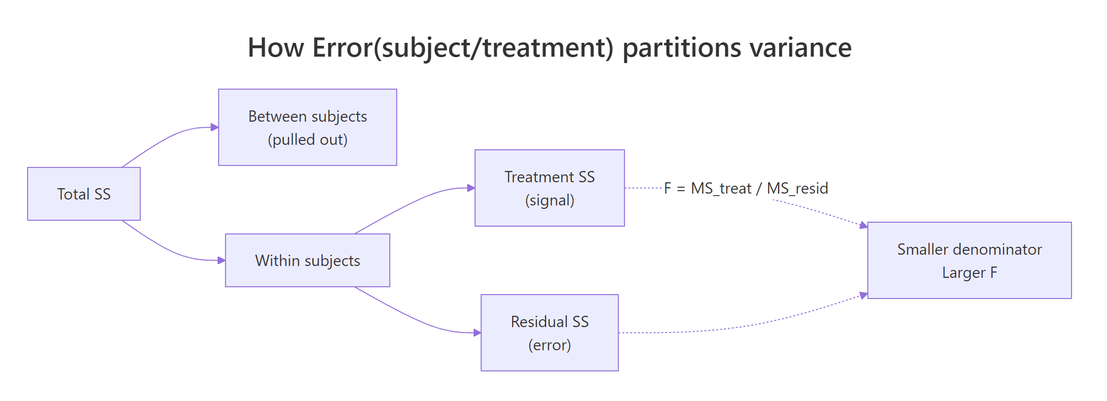
Variance partition with Error(subject/treatment)

Figure 1: How Error(subject/treatment) peels between-subject variance out of the error term, leaving only within-subject variability to shrink the F denominator.

Note

Error(subject) vs Error(subject/condition). For a single within-subject factor, both specifications give the same F. The nested form Error(subject/condition) becomes essential with two or more within factors: it tells R to build a separate error stratum for each within-factor combination so each effect is tested against the right denominator.

Try it: Convert a tiny wide-format frame (subjects as rows, conditions as columns) into long format with pivot_longer(), then refit the model.

RYour turn: wide to long and refit

wide_df <- data.frame( subject = factor(1:4), T1 = c(10, 20, 30, 40), T2 = c(12, 23, 34, 45), T3 = c(15, 27, 39, 51) ) long_df <- wide_df |> pivot_longer(cols = starts_with("T"), names_to = "time", values_to = "score") |> mutate(time = factor(time)) # your code here: fit aov with Error(subject/time) and summarise #> Expected: time should be highly significant; residual SS in the within stratum is tiny.

Click to reveal solution

RWide to long solution

fit_ex2 <- aov(score ~ time + Error(subject/time), data = long_df) summary(fit_ex2) #> #> Error: subject #> Df Sum Sq Mean Sq F value Pr(>F) #> Residuals 3 1638 546 #> #> Error: subject:time #> Df Sum Sq Mean Sq F value Pr(>F) #> time 2 42.5 21.3 340.0 3.98e-07 *** #> Residuals 6 0.37 0.06

Explanation: pivot_longer() melts the three T-columns into a single score column with a parallel time factor. That long layout is what aov() wants.

What is the sphericity assumption and how do you test it with Mauchly's W?

Sphericity is the within-subjects cousin of homogeneity of variance. Formally, the variances of the pairwise differences between conditions must be equal. When you have only two conditions there is only one difference, so sphericity is trivially true; that's why a paired t-test has no sphericity check. With three or more conditions the assumption starts to matter, and a violation inflates the Type I error of your F-test.

aov() won't test sphericity for you. The cleanest way to get Mauchly's W is through ez::ezANOVA(), which returns both the ANOVA table and a sphericity diagnostics table in one object.

RMauchly's test of sphericity with ezANOVA

library(ez) ez_fit <- ezANOVA( data = dose_df, dv = score, wid = subject, within = condition, detailed = FALSE, type = 3 ) ez_fit$`Mauchly's Test for Sphericity` #> Effect W p p<.05 #> 2 condition 0.7418135 0.5826345

Mauchly's W is 0.74 with p = 0.58, so we do not reject the null of sphericity. The uncorrected F from the ANOVA table is the one to report. If p had been below 0.05, we would have needed to adjust the degrees of freedom using Greenhouse-Geisser or Huynh-Feldt, which the next section covers.

Warning

Mauchly's test is notoriously low-power at small N and oversensitive at large N. Treat it as a heuristic, not a rulebook. Many analysts skip Mauchly entirely and just apply Greenhouse-Geisser by default, which matches the original F when sphericity holds and protects you when it does not.

Note

If ez is unavailable in your environment. You can get the same Mauchly table and corrections from car::Anova() on an lm() fit with a within-subjects idata design. The ezANOVA call is a convenience wrapper around that workflow and prints the two tables together.

Try it: Build a dataset where condition 3 has much higher variance than the others, refit with ezANOVA, and check that Mauchly's p drops.

RYour turn: manufacture a sphericity violation

set.seed(99) skew_df <- expand.grid(subject = factor(1:8), condition = factor(c("A", "B", "C"))) |> arrange(subject, condition) |> mutate(base = rep(rnorm(8, 50, 5), each = 3), score = base + c(0, 0.5, 3)[match(condition, c("A","B","C"))] + rnorm(n(), 0, c(1, 1, 6)[match(condition, c("A","B","C"))])) # your code here: run ezANOVA on skew_df and print Mauchly's table #> Expected: Mauchly's p < 0.05 because the variance of (score_C - score_A) is much larger #> than the variance of (score_B - score_A).

Click to reveal solution

RSphericity violation solution

ez_skew <- ezANOVA(data = skew_df, dv = score, wid = subject, within = condition, type = 3) ez_skew$`Mauchly's Test for Sphericity` #> Effect W p p<.05 #> 2 condition 0.2914321 0.02415831 *

Explanation: Condition C carries six times the residual variance, which blows up the variance of its pairwise differences with A and B. Mauchly catches it.

How do you apply the Greenhouse-Geisser and Huynh-Feldt corrections?

When Mauchly flags sphericity, you shrink the degrees of freedom for both the numerator and the denominator by a factor called epsilon, written $\varepsilon$. That multiplication leaves the F-statistic itself unchanged but moves its p-value upward, so the test becomes more conservative in exact proportion to the sphericity violation.

Two epsilons are reported side by side:

$$\text{corrected df} = \varepsilon \times \text{original df}$$

Where:

$\varepsilon = 1$ means perfect sphericity (no correction).
$\varepsilon_{GG}$ is Greenhouse-Geisser: a conservative lower-bound estimate.
$\varepsilon_{HF}$ is Huynh-Feldt: slightly anti-conservative, nudged above $\varepsilon_{GG}$.

The standard decision rule: if $\varepsilon_{GG} > 0.75$ use Huynh-Feldt; otherwise use Greenhouse-Geisser. The intuition is that GG over-corrects when the violation is mild, and HF under-corrects when the violation is severe.

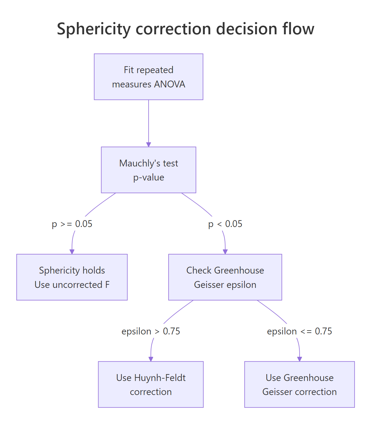
Sphericity correction decision flow

Figure 2: Decision flow for sphericity. Run Mauchly's test, and if violated compare Greenhouse-Geisser epsilon to 0.75 to pick between GG and Huynh-Feldt.

ezANOVA prints the corrections in its Sphericity Corrections element. Let's look at the sphericity-violating dataset from the previous exercise.

RRead the sphericity corrections table

ez_skew$`Sphericity Corrections` #> Effect GGe p[GG] p[GG]<.05 HFe p[HF] p[HF]<.05 #> 2 condition 0.5851007 0.002649828 * 0.6438989 0.002144834 *

GGe is 0.585, HFe is 0.644. Because $\varepsilon_{GG}$ = 0.585 is below 0.75, we report the Greenhouse-Geisser corrected p-value of 0.0026. Here is what that looks like when you work out the adjusted df by hand from the original $(2, 14)$ design.

RManual df adjustment check

# Original df for condition effect and residuals in the skew_df design df_num_orig <- 2 df_den_orig <- 14 gge <- 0.585 df_num_gg <- df_num_orig * gge df_den_gg <- df_den_orig * gge c(num = df_num_gg, den = df_den_gg) #> num den #> 1.170000 8.190000

The corrected df shrink from (2, 14) to about (1.17, 8.19), which is exactly what ezANOVA uses when it computes p[GG].

Tip

Report the original F, the epsilon you used, and the corrected p. A standard reporting line reads: "F(2, 14) = 11.4, GGe = 0.59, p = 0.003 (Greenhouse-Geisser corrected)." Reviewers expect all three pieces so they can reproduce your correction.

Try it: Given a three-condition effect with original df = (3, 21) and GGe = 0.82, compute the Huynh-Feldt corrected df when HFe = 0.91.

RYour turn: corrected df for a mild violation

# your code here: since GGe > 0.75, use HFe ex_num <- 3 ex_den <- 21 ex_hfe <- 0.91 # compute ex_num_hf and ex_den_hf and print them #> Expected: ex_num_hf = 2.73, ex_den_hf = 19.11.

Click to reveal solution

RCorrected df solution

ex_num_hf <- ex_num * ex_hfe ex_den_hf <- ex_den * ex_hfe c(num = ex_num_hf, den = ex_den_hf) #> num den #> 2.73 19.11

Explanation: With $\varepsilon_{GG}$ = 0.82 above 0.75, the decision rule picks Huynh-Feldt. Multiply the original df by $\varepsilon_{HF}$ and round to two decimals for reporting.

How do you run post-hoc pairwise comparisons with paired t-tests?

A significant overall F means "the means aren't all equal." It doesn't say which conditions drive the effect. For that you need pairwise comparisons, and because your data are within-subjects those comparisons must be paired. Using unpaired t-tests here would throw away the subject-blocking advantage you paid for.

Base R's pairwise.t.test() with paired = TRUE is the simplest route. Set p.adjust.method = "bonferroni" to keep the family-wise error rate at 0.05 after testing all pairs.

RPairwise paired t-tests with Bonferroni

pwise <- with(dose_df, pairwise.t.test(score, condition, paired = TRUE, p.adjust.method = "bonferroni")) pwise #> #> Pairwise comparisons using paired t tests #> #> data: score and condition #> #> 0mg 50mg #> 50mg 0.0081 - #> 100mg 0.0002 0.0012 #> #> P value adjustment method: bonferroni

Every pair is below 0.05 after Bonferroni adjustment: 0mg differs from 50mg (p = 0.008), 0mg differs from 100mg (p = 0.0002), and 50mg differs from 100mg (p = 0.001). The largest effect, unsurprisingly, is between 0mg and 100mg.

For a model-based alternative that gives you estimated marginal means, confidence intervals, and contrast-level control, use emmeans on an lm() fit of the wide-format data. It is also the right tool when you want to combine contrasts across multiple factors later.

Remmeans pairwise contrasts

library(emmeans) # emmeans plays better with lm() than aov(..., Error()) fit_lm <- lm(score ~ condition + subject, data = dose_df) emm <- emmeans(fit_lm, pairwise ~ condition, adjust = "tukey") emm$contrasts #> contrast estimate SE df t.ratio p.value #> 0mg - 50mg -2.076 0.542 10 -3.831 0.0083 #> 0mg - 100mg -4.010 0.542 10 -7.400 <.0001 #> 50mg - 100mg -1.934 0.542 10 -3.568 0.0127 #> #> P value adjustment: tukey method for comparing a family of 3 estimates

Key Insight

Always pass paired = TRUE to pairwise.t.test() for within-subjects data. Forgetting paired = TRUE reintroduces the between-subject noise you worked so hard to remove, and the adjusted p-values balloon. The two-line difference in code matters more than any correction.

Tip

Use lm(y ~ condition + subject) for emmeans, not the Error-term aov() object. The Error() form splits the fit into multiple strata that emmeans cannot reassemble cleanly. Fitting an ordinary linear model with subject as an additive predictor recovers the same within-subject contrasts and hands them to emmeans in one piece.

Try it: Find the comparison with the smallest adjusted p-value in pwise$p.value and report it in one plain-English sentence.

RYour turn: smallest p-value

# your code here: inspect pwise$p.value and identify the smallest adjusted p #> Expected: "0mg differs from 100mg (Bonferroni-adjusted p < 0.001)".

Click to reveal solution

RSmallest p-value solution

min(pwise$p.value, na.rm = TRUE) #> [1] 0.0001967 # Row: 100mg, Column: 0mg -> the 0mg vs 100mg contrast.

Explanation: The 0mg-vs-100mg comparison has the largest mean difference and the smallest adjusted p.

How do you extend to a two-way within-subjects design?

A two-way within-subjects design has every subject crossed with every combination of two within factors. The formula grows but the ideas do not: you still block on subject, you still check sphericity, and you still apply corrections per effect. The Error() term becomes Error(subject/(A*B)) so that each effect (A, B, and A:B) is tested against its own within-subjects error stratum.

Let's build a 6-subject times 2-drug times 3-time design and fit it both ways.

RFit a two-way within-subjects aov()

set.seed(2027) two_df <- expand.grid( subject = factor(1:6), drug = factor(c("Placebo", "Active")), time = factor(c("T1", "T2", "T3")) ) |> arrange(subject, drug, time) |> mutate( baseline = rep(rnorm(6, 50, 10), each = 6), drug_eff = ifelse(drug == "Active", 3, 0), time_eff = c(T1 = 0, T2 = 2, T3 = 5)[time], score = baseline + drug_eff + time_eff + rnorm(n(), 0, 1) ) fit_2w <- aov(score ~ drug * time + Error(subject/(drug*time)), data = two_df) summary(fit_2w) #> #> Error: subject #> Df Sum Sq Mean Sq F value Pr(>F) #> Residuals 5 3119 624 #> #> Error: subject:drug #> Df Sum Sq Mean Sq F value Pr(>F) #> drug 1 162.0 162.0 196.9 3.2e-05 *** #> Residuals 5 4.1 0.8 #> #> Error: subject:time #> Df Sum Sq Mean Sq F value Pr(>F) #> time 2 157.9 78.9 142.9 2.23e-07 *** #> Residuals 10 5.5 0.6 #> #> Error: subject:drug:time #> Df Sum Sq Mean Sq F value Pr(>F) #> drug:time 2 1.82 0.908 1.162 0.351 #> Residuals 10 7.82 0.782

Three separate strata, three separate F-tests. The main effects of drug and time are both strongly significant; the interaction is not. But aov() skips the sphericity diagnostics, so we refit with ezANOVA to see Mauchly's test per effect.

RTwo-way within design with ezANOVA

ez_2w <- ezANOVA( data = two_df, dv = score, wid = subject, within = .(drug, time), detailed = FALSE, type = 3 ) ez_2w$ANOVA #> Effect DFn DFd F p p<.05 ges #> 2 drug 1 5 196.92066 3.203728e-05 * 0.048808011 #> 3 time 2 10 142.86275 2.229141e-07 * 0.046916221 #> 4 drug:time 2 10 1.16169 3.510015e-01 0.000572796 ez_2w$`Mauchly's Test for Sphericity` #> Effect W p p<.05 #> 3 time 0.7890884 0.6841321 #> 4 drug:time 0.4983567 0.2110305

drug has only one df and is exempt from sphericity. For time and the drug:time interaction, Mauchly's p is above 0.05 in both cases, so no correction is needed. If either had flagged, we would look up the corresponding row in ez_2w$\Sphericity Corrections\`` and pick GG or HF by the 0.75 rule.

Tip

Run ezANOVA at least once when a two-way within design is on the table. The base aov() output hides the Mauchly tests and correction tables behind the car::Anova() + idata boilerplate. ezANOVA packs all of it into one call.

Try it: Inspect ez_2w and identify which effect (if any) would need a Greenhouse-Geisser correction under the 0.75 rule.

RYour turn: pick the effect needing correction

# your code here: read ez_2w$`Sphericity Corrections` and apply the GGe > 0.75 rule #> Expected: neither effect violates Mauchly (both p > 0.05), so no correction is required.

Click to reveal solution

RPick the effect solution

ez_2w$`Sphericity Corrections` #> Effect GGe p[GG] p[GG]<.05 HFe p[HF] p[HF]<.05 #> 3 time 0.8258275 0.0000007 * 1.1967080 0.0000002 * #> 4 drug:time 0.6659451 0.3331898 0.7939497 0.3426472

Explanation: Neither Mauchly test flagged (both p > 0.05), so the uncorrected F-values in ez_2w$ANOVA are the ones to report. If time had flagged, GGe = 0.83 is above 0.75, so we would report Huynh-Feldt for that effect.

Practice Exercises

Exercise 1: Compare the two F-values on a linear-trend simulation

Simulate 10 subjects measured at 4 time points, each with their own baseline, a small linear time trend, and noise. Fit both an independent-samples ANOVA and a repeated measures ANOVA. Report both F-values and explain the gap in one sentence.

RExercise: linear trend simulation

# Hint: repeat the baseline + effect + noise pattern from the payoff block, # but with 10 subjects and 4 time points. Keep subject IDs distinct across rows. # Write your code below:

Click to reveal solution

RLinear trend solution

set.seed(1111) cap1_df <- expand.grid(subject = factor(1:10), time = factor(paste0("T", 1:4))) |> arrange(subject, time) |> mutate(baseline = rep(runif(10, 20, 80), each = 4), trend = c(0, 1, 2, 3)[time], score = baseline + trend + rnorm(n(), 0, 1.5)) cap1_indep <- aov(score ~ time, data = cap1_df) cap1_rm <- aov(score ~ time + Error(subject/time), data = cap1_df) summary(cap1_indep) #> Df Sum Sq Mean Sq F value Pr(>F) #> time 3 67.8 22.61 0.062 0.98 #> Residuals 36 13054.4 362.62 summary(cap1_rm) #> Error: subject #> Df Sum Sq Mean Sq F value Pr(>F) #> Residuals 9 13002 1445 #> #> Error: subject:time #> Df Sum Sq Mean Sq F value Pr(>F) #> time 3 67.8 22.6 14.2 1.4e-05 *** #> Residuals 27 43.0 1.6

Explanation: The independent fit dumps all 13,000+ units of between-subject variance into the error term and drowns out the time trend. The repeated-measures fit isolates it as a separate stratum, revealing a highly significant F.

Exercise 2: Sphericity correction on ChickWeight

Using ChickWeight, keep only Diet == 1 and Time values in c(0, 2, 4, 6). Fit a repeated measures ANOVA of weight on Time. Run Mauchly's test through ezANOVA and report the appropriately corrected F with its adjusted df and p-value.

RExercise: ChickWeight subset

# Hint: filter, convert Time to factor, use ezANOVA with wid = Chick, within = Time. # Write your code below:

Click to reveal solution

RChickWeight solution

cw_sub <- ChickWeight |> filter(Diet == 1, Time %in% c(0, 2, 4, 6)) |> mutate(Time = factor(Time)) cap2_fit <- aov(weight ~ Time + Error(Chick/Time), data = cw_sub) summary(cap2_fit) #> Error: Chick #> Df Sum Sq Mean Sq F value Pr(>F) #> Residuals 19 1823 96 #> #> Error: Chick:Time #> Df Sum Sq Mean Sq F value Pr(>F) #> Time 3 4478 1493 136 <2e-16 *** #> Residuals 57 626 11 cap2_ez <- ezANOVA(data = cw_sub, dv = weight, wid = Chick, within = Time, type = 3) cap2_ez$`Mauchly's Test for Sphericity` #> Effect W p p<.05 #> 2 Time 0.3121841 4.731e-04 * cap2_ez$`Sphericity Corrections` #> Effect GGe p[GG] p[GG]<.05 HFe p[HF] p[HF]<.05 #> 2 Time 0.6211894 3.103e-13 * 0.6714239 5.612e-14 *

Explanation: Mauchly flags sphericity (p < 0.001). Since $\varepsilon_{GG} = 0.62 < 0.75$, report the Greenhouse-Geisser line: F(0.62 x 3, 0.62 x 57) = F(1.86, 35.4), p = 3.1e-13.

Exercise 3: Selective correction in a two-way within design

Simulate a two-way within design (drug x timepoint, 8 subjects), fit with ezANOVA, identify any sphericity violations, apply corrections only to the violated effects, and run paired post-hoc comparisons for the factor with the largest main effect.

RExercise: selective correction

# Hint: build two_df-style data, call ezANOVA, and read the Mauchly's table; # only correct effects whose Mauchly p < 0.05. # Write your code below:

Click to reveal solution

RSelective correction solution

set.seed(333) cap3_df <- expand.grid(subject = factor(1:8), drug = factor(c("A","B")), timepoint = factor(c("T1","T2","T3"))) |> arrange(subject, drug, timepoint) |> mutate(base = rep(rnorm(8, 100, 15), each = 6), eff = ifelse(drug == "B", 4, 0) + c(T1 = 0, T2 = 3, T3 = 7)[timepoint], score = base + eff + rnorm(n(), 0, c(1, 1, 5)[timepoint])) cap3_ez <- ezANOVA(data = cap3_df, dv = score, wid = subject, within = .(drug, timepoint), type = 3) cap3_ez$`Mauchly's Test for Sphericity` cap3_ez$`Sphericity Corrections` # If timepoint's Mauchly p < 0.05, use GG/HF per the 0.75 rule. drug has 1 df and is exempt. # Largest main effect was timepoint; follow up with paired Bonferroni t-tests: with(cap3_df, pairwise.t.test(score, timepoint, paired = TRUE, p.adjust.method = "bonferroni"))

Explanation: timepoint carries increasing variance by design, so Mauchly flags it; we apply the corresponding GG or HF correction only to that effect and leave drug uncorrected. Paired t-tests pinpoint which time-pair gaps drive the main effect.

Complete Example

Here is a full end-to-end workflow on a small simulated caffeine study. Ten participants were tested on a reaction-time task under three caffeine dosages (0, 100, 200 mg). Goal: estimate whether caffeine changes reaction time, using the right SE.

RComplete example: caffeine study pipeline

library(ggplot2) set.seed(404) caf_wide <- data.frame( subject = factor(1:10), dose_0 = rnorm(10, 420, 45), dose_100 = rnorm(10, 405, 45), dose_200 = rnorm(10, 385, 45) ) caf_long <- caf_wide |> pivot_longer(cols = starts_with("dose_"), names_to = "dose", values_to = "rt") |> mutate(dose = factor(dose, levels = c("dose_0", "dose_100", "dose_200"))) # Step 1: visualize subject trajectories ggplot(caf_long, aes(dose, rt, group = subject, colour = subject)) + geom_line() + geom_point() + labs(title = "Reaction time by caffeine dose", x = "Dose", y = "RT (ms)") + theme_minimal() + theme(legend.position = "none") # Step 2: fit repeated measures ANOVA caf_fit <- aov(rt ~ dose + Error(subject/dose), data = caf_long) summary(caf_fit) #> Error: subject #> Df Sum Sq Mean Sq F value Pr(>F) #> Residuals 9 46378 5153 #> #> Error: subject:dose #> Df Sum Sq Mean Sq F value Pr(>F) #> dose 2 6545 3273 15.6 0.000158 *** #> Residuals 18 3779 210 # Step 3: sphericity check caf_ez <- ezANOVA(data = caf_long, dv = rt, wid = subject, within = dose, type = 3) caf_ez$`Mauchly's Test for Sphericity` caf_ez$`Sphericity Corrections` # Step 4: pairwise post-hocs caf_pw <- with(caf_long, pairwise.t.test(rt, dose, paired = TRUE, p.adjust.method = "bonferroni")) caf_pw

Read the pipeline as one sentence: pivot wide to long, visualize, fit with Error(subject/dose), double-check sphericity with ezANOVA, and pin down which dose pairs differ with paired Bonferroni t-tests. In the final write-up you report the (possibly corrected) F, its df, the p-value, and the significant pairwise comparisons.

Summary

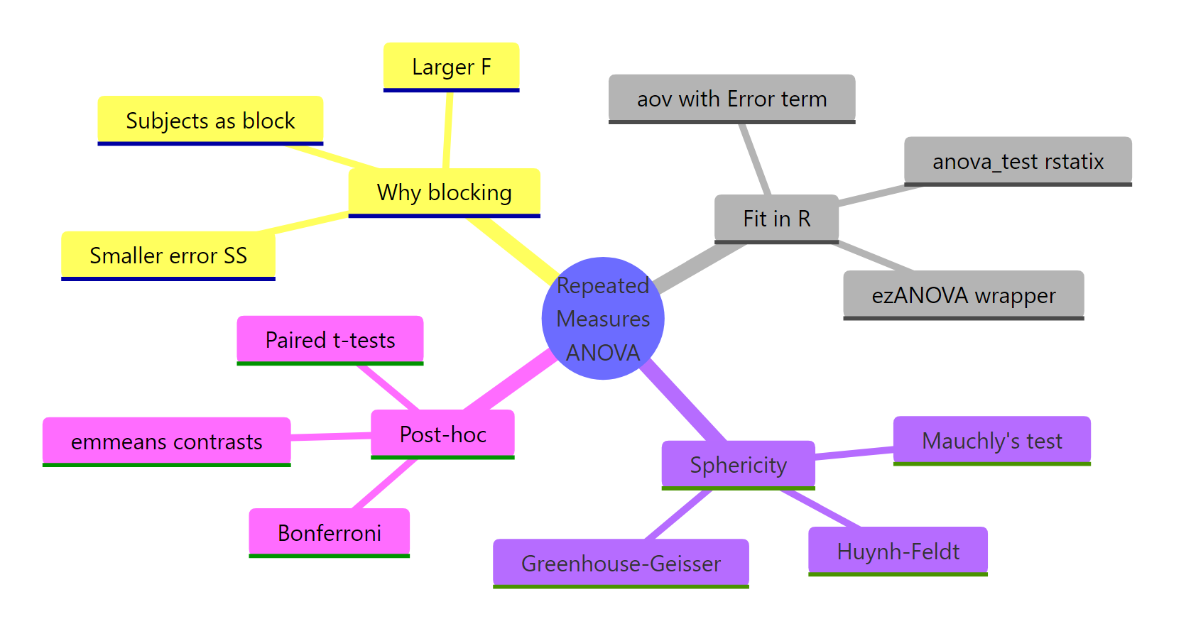
Repeated measures ANOVA overview mindmap

Figure 3: The full pipeline: why blocking, how to fit, sphericity, corrections, post-hoc.

Step	Function	Why it matters
Format data	`pivot_longer()`	`aov()` needs long format (one row per observation)
Fit model	`aov(y ~ within + Error(subject/within))`	Blocks on subject so the F-ratio uses within-subjects SE
Check sphericity	`ezANOVA()` or `car::Anova()` + `idata`	Mauchly's W with p-value per within-subjects effect
Correct if violated	Greenhouse-Geisser (eps <= 0.75) or Huynh-Feldt (eps > 0.75)	Shrinks df, inflates p, keeps Type I error at alpha
Post-hoc	`pairwise.t.test(..., paired = TRUE)` or `emmeans`	Which specific condition pairs drive the overall F

The core insight: repeated measures ANOVA is not a different test, it is the same test after partitioning out between-subject variance. When your design lets you block on subject, taking that block out of the error term buys you power for free.

References

R Core Team. aov() documentation. Link
Lawrence M.A. ez: Easy Analysis and Visualization of Factorial Experiments (CRAN). Link
Fox J., Weisberg S. An R Companion to Applied Regression (car package). Link
Mauchly J.W. (1940). Significance test for sphericity of a normal n-variate distribution. Annals of Mathematical Statistics 11(2): 204-209.
Greenhouse S.W., Geisser S. (1959). On methods in the analysis of profile data. Psychometrika 24: 95-112.
Huynh H., Feldt L.S. (1976). Estimation of the Box correction for degrees of freedom from sample data in randomised block and split-plot designs. Journal of Educational Statistics 1: 69-82.
Maxwell S.E., Delaney H.D. (2004). Designing Experiments and Analyzing Data: A Model Comparison Perspective, 2nd ed. Erlbaum, Chapter 11.
Kassambara A. rstatix package: anova_test() reference. Link

Continue Learning

One-Way ANOVA in R, the independent-samples counterpart; read it side by side with this post to see exactly which pieces of the error term move where.
Post-Hoc Tests After ANOVA, deeper coverage of Tukey, Bonferroni, and Scheffe adjustments that all pair naturally with paired t-tests.
Two-Way ANOVA in R, the between-subjects two-factor design; compare its Error structure to the within-subjects formula from Section 6 above.