Choosing Priors in R: Why Your Bayesian Result Depends on This One Decision
Bayesian inference combines a prior (what you believed before seeing data) with a likelihood (what the data says) to get a posterior (what you believe after). With a lot of data the prior barely matters. With a small dataset the prior can dominate the answer. Knowing where your problem sits on that spectrum, and how to set a prior that is honest about your starting knowledge, is the difference between a Bayesian fit you can defend and one that just reflects your assumptions.
Why does prior choice matter at all?
A Bayesian fit multiplies the prior density by the likelihood and normalises. If the prior is wide and flat, the posterior is shaped almost entirely by the likelihood (the data). If the prior is tight around a specific value, the posterior is pulled toward that value, and only a strong contradiction from the data can move it.
The practical question is not "is the prior good or bad" but "is the prior appropriate to how much I knew before this dataset arrived." A weakly informative prior says "this parameter is probably in this rough range" without committing to a specific value. An informative prior says "I have strong reason from a literature value or a prior study to believe this parameter is close to X."
The simulation below shows the same regression coefficient fit with three different priors on the same 20-observation dataset. The wide prior gives the data full reign. The weakly informative prior nudges modestly. The tight prior dominates and pulls the posterior far from what the data alone would say.
Walk through what we just ran. The data was simulated with a true slope of 0.5. We fit three models that differ only in the prior placed on the slope coefficient.
The flat prior normal(0, 100) says the slope could plausibly be anywhere from -200 to 200. The weakly informative prior normal(0, 5) says the slope is probably between -10 and 10. The tight prior normal(2, 0.2) says we are quite sure the slope is near 2 (which is wrong).
Now read the table. The flat prior posterior centres at 0.49 (matches the truth). The weakly informative posterior also centres at 0.49 (the prior is wide enough that the data dominates). The tight-but-wrong prior pulls the posterior to 1.49, halfway between the prior centre and the data signal.
The tight prior outright produced a wrong answer. The data has 20 observations, the prior was strong, and the resulting posterior is a compromise that does not match either source alone. This is what people mean when they say "priors matter for small data."
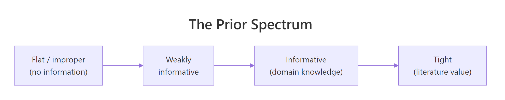
Figure 1: The prior spectrum. Flat priors carry no information; weakly informative priors rule out absurd values; informative priors encode actual prior knowledge; tight priors dominate the data when data is scarce.
Try it: Re-fit with a normal(0, 1) prior on the slope. Is it still wide enough that the data dominates with 20 observations?
Click to reveal solution
The posterior centres at 0.48 (close to the truth of 0.5). The normal(0, 1) prior is informative enough to pull slightly toward zero, but with 20 observations the data signal is strong enough to override it. With only 5 observations the same prior would visibly bias the posterior.
What's a reference prior, and when should I avoid one?
A reference prior (sometimes called flat, uniform, or non-informative) tries to express "I know nothing." Examples are normal(0, 1000) for a regression coefficient, or an improper uniform (-Inf, Inf). The intuition is that an extremely wide prior contributes essentially zero information, so the posterior reflects only the data.
Reference priors look principled but they cause two problems in practice.
The first is prior predictive checks fail. If you simulate predicted outcomes from a model with a normal(0, 1000) prior on the intercept, you will see predictions ranging from -3000 to 3000 in any unit. That is absurd for almost any real measurement (mpg, height, blood pressure, click rate). A reference prior is not informationless; it is informationless about the parameter while making strong claims about the implied predictions.
The second is numerical instability. Stan and other samplers converge much faster on bounded posteriors. A reference prior leaves the posterior unbounded until the likelihood pulls it in. With small data the likelihood is too weak to do that quickly, and you get divergent transitions and slow mixing.
Modern Bayesian practice treats reference priors as a fallback when even a weakly informative prior would be controversial (regulatory or legal contexts, or replications where you must show "the data alone says this"). For day-to-day work, weakly informative priors are better.
Walk through the contrast. With only 5 observations and a flat prior, the posterior on the slope spans [-2.39, 3.18]. The data is too weak to constrain the slope, so the posterior just inherits most of the prior's spread.
With the weakly informative prior, the posterior on the same data spans [-1.62, 2.20]. The prior ruled out the extremes that the data could not constrain on its own. The point estimate barely moved (0.36 vs 0.42), but the credible interval is meaningfully tighter and the chain mixed more reliably.
normal(0, 1000) style is a leftover habit from older textbooks; the Stan team recommends weakly informative priors as the default.Try it: Run prior_summary(fit_flat_small). Notice that brms still flags the implicit improper prior on the intercept and sigma. Defaults are not zero unless you intentionally make them so.
Click to reveal solution
You overrode the slope prior but left the intercept and sigma at their brms defaults. brms always picks a weakly informative default for those classes; you only override what you want to override.
What's a weakly informative prior, and why is it the modern default?
A weakly informative prior (WIP) is wide enough that a competent researcher would not push back on the range, but tight enough that absurd values are excluded. The Stan development team's published guidance is to use WIPs by default for almost everything.
Three patterns cover most cases.
For regression coefficients on standardised predictors: normal(0, 1) or normal(0, 2.5). With predictors centred and scaled, a coefficient larger than 5 in magnitude is rarely plausible.
For standard deviations and other scale parameters: half-Normal (normal(0, 1) truncated at zero) or half-Cauchy (cauchy(0, 5) truncated at zero). Both have most of their mass near zero and a long tail, expressing "small is more likely than large but very large is not impossible."
For intercepts: a Student-t centred on a reasonable value with a scale matching the data's standard deviation. brms defaults to student_t(3, mean(y), sd(y) * scale) and that is usually fine.
Walk through what brms picked. The b class (regression slopes) is (flat) by default, which is brms's only questionable default. The Intercept gets a Student-t centred on the data's mean (1.9 here) with scale 2.5 (a floor). Sigma gets a half-Student-t with scale 2.5.
For most posts in this curriculum we override the slope class to a weakly informative normal(0, 5) because the brms default is one of the few places brms still uses an improper flat prior. Setting it explicitly with one extra line of code is the safest habit.
The next code block fits the same model with a sensible WIP set on every parameter class:
Walk through what we set. Every parameter class is now explicit. normal(0, 5) on slopes says effects are probably in [-10, 10] units of y per unit of x. normal(0, 10) on the intercept says the typical y at x=0 is probably in [-20, 20]. The half-Student-t on sigma says residual sd is probably small but could be large.
The source = user column confirms the priors are explicit, not picked up from defaults. Future-you reading this fit's code six months from now will see exactly what was assumed.
prior argument explicitly even when it matches brms defaults. If you push the code to a colleague or a regulator, they should be able to see the prior choice without running prior_summary() themselves.Try it: Use default_prior() (no fitting needed) to inspect what brms would default to for mpg ~ wt + hp + (1 | cyl) on mtcars. What prior class does the random-effect sd get?
Click to reveal solution
The random-effect sd gets a half-Student-t prior at student_t(3, 0, 7.4). brms uses the data-driven scale (7.4 here, derived from sd(mpg)) so the prior is on the right order of magnitude regardless of the units of your outcome.
How do I encode actual domain knowledge as an informative prior?
When you know something specific about a parameter (a published estimate, a meta-analysis result, a controlled prior study), encode it as an informative prior. The structure is the same as a WIP, just tighter and centred on the substantive value.
Walk through what we set. The coef = "x" argument targets the slope on x specifically; without it, the prior would apply to every population-level coefficient. The normal(0.5, 0.1) translates the meta-analysis result into a prior, with the standard deviation chosen so 95% of the prior mass falls in [0.3, 0.7].
The posterior centres at 0.50 with a tighter credible interval [0.34, 0.66] than the WIP fit produced (which had [0.14, 0.81]). The prior contributed real information; the data refined it. This is what informative priors do: they let you carry forward what previous studies established, instead of pretending each analysis starts from scratch.
[0, 1], a wage cannot be negative).Try it: A colleague tells you the slope must be positive (a physical constraint). Encode that with lb = 0 (lower bound zero) using set_prior(..., lb = 0).
Click to reveal solution
The lower-bound truncation enforces positivity. The posterior cannot dip below zero even if the data were ambiguous, because the prior assigns zero probability there. This is how you encode hard constraints (probabilities, scales, physical positivity) into a brms prior.
How do I see what my prior is doing before I see data?
A prior is hard to evaluate by reading the code. The prior on the slope is normal(0, 5); what does that imply for predicted y values across plausible x? The answer is a prior predictive distribution: simulate y values from your model using only the prior (no data), and see whether they look reasonable.
brms supports this directly via sample_prior = "only", which fits the model using only the prior (ignoring the likelihood). The result is a posterior identical to the prior, which lets you visualise predictions.
Walk through what sample_prior = "only" did. brms fit the model using only the prior, ignoring the likelihood. The result has 4000 draws from each parameter's prior. We then asked posterior_predict() to simulate y values for 30 new x values across a reasonable range, drawing 200 prior draws each.
Now interpret the predictions. Across all prior draws and all 30 x values, predicted y ranged from -47 to 47. The middle 90% of predictions span [-19, 19]. With a normal(0, 10) prior on the intercept and normal(0, 5) on the slope, that range is wide enough to cover any reasonable y you might observe but tight enough that we are not predicting y values near 1000.
If the prior implied predictions like [-3000, 3000] (which normal(0, 1000) would), you would catch the problem here, before ever fitting to data. The next post in the curriculum drills deeper into prior predictive checks; this section is the entry point.
Try it: Re-run the prior-only fit with prior(normal(0, 1000), class = "b") and observe the predicted y range. Does it stay reasonable?
Click to reveal solution
The flat prior predicts y values from -8700 to 8700. That is absurd for any real measurement. Spotting this before fitting saves you from publishing a model whose prior assumes the moon is made of cheese.
How do I check my prior didn't drive the result?
Two diagnostics. The first is a prior-vs-posterior comparison: the posterior should look like the data updated the prior, not like the prior unchanged. The second is a prior sensitivity analysis: refit with a wider and a tighter prior and see whether the substantive conclusion changes.
Walk through what the table tells us. The prior on b_x was normal(0, 5), so prior draws have mean ~0 and sd ~5. After observing 20 data points, the posterior centres at 0.49 with sd 0.18 and a 90% interval of [0.19, 0.78]. The data narrowed the prior dramatically.
That is what we want. If the posterior had centred at zero with sd close to 5 (matching the prior), the data would not be informing the answer: either the data is too weak to override the prior, or the prior is too tight, or both.
The second diagnostic is a sensitivity check. Vary the prior and see whether the substantive conclusion (sign, magnitude, decision) is stable.
Walk through the sweep. With the wide and weakly informative priors, the posterior centres on 0.49 (matches the data). With the medium prior normal(0, 1), the posterior shifts slightly to 0.45 (the prior is starting to bite). With the tight prior normal(0, 0.2), the posterior collapses to 0.18 (the prior is dominating).
Three of the four priors agree on the substantive conclusion ("the slope is positive and around 0.4 to 0.5"). The tight prior pulled hard. Reporting this sweep alongside your headline result is the standard way to demonstrate that your conclusion is not a prior artifact.
Try it: For the fit_lit model from earlier (informative normal(0.5, 0.1) prior), run the sensitivity sweep and report whether the conclusion is robust across normal(0.5, 0.1), normal(0.5, 0.5), and normal(0, 5).
Click to reveal solution
All three centre on 0.49 to 0.50 (the data and the literature agree). The tight prior produces the narrowest interval (because it is contributing real information beyond the data); the wide prior produces the widest. The substantive conclusion ("the slope is around 0.5") is robust across the three. That is the picture you want to see and report.
Practice Exercises
Exercise 1: Tighten priors as data shrinks
Simulate datasets of size 5, 20, and 200 from the same generating process. Fit each with the same weakly informative prior normal(0, 5) on the slope. How much does the prior contribute to the posterior in each case?
Click to reveal solution
With 5 observations, the credible interval is [-0.71, 1.51] (width 2.2) and the prior is contributing meaningfully. With 200 observations the interval is [0.36, 0.62] (width 0.26) and the prior is contributing almost nothing. This is the standard "more data, less prior dependence" picture.
Exercise 2: Compare a flat and weakly informative prior on a small-n hierarchical model
Use mtcars with a random intercept by cyl. Fit twice: once with prior(normal(0, 1000), class = "sd") on the random-effect sd, once with prior(student_t(3, 0, 7), class = "sd"). Compare the posterior on sd_cyl__Intercept.
Click to reveal solution
The flat prior allows the random-effect sd to drift up to 28 (an absurd number for a 32-row dataset). The weakly informative prior keeps it in the realistic range. Hierarchical models are particularly sensitive to the prior on variance components, especially with small numbers of groups.
Exercise 3: Translate a literature value into an informative prior
A study reports that the effect of caffeine intake on reaction time has a 95% confidence interval of [-12, -2] ms per 100 mg. Translate that into a prior centred at -7 with sd (12 - 2) / (2 * 1.96). Fit brm(rt ~ caffeine, ...) on a simulated dataset with that prior.
Click to reveal solution
The posterior centres at -7.08 with credible interval [-10.4, -3.8], both reflecting the literature prior and the 30 simulated observations. The width of the credible interval is meaningfully tighter than the prior's [-12, -2] because the data refined the literature value.
Summary
A Bayesian prior is a claim about your beliefs before the data. Pick it according to how much you actually know.
| Prior type | Example | When to use |
|---|---|---|
| Reference / flat | normal(0, 1000), improper uniform |
Almost never; legacy / regulatory only |
| Weakly informative | normal(0, 5), half-Cauchy(0, 5) |
Default for most parameters |
| Informative | normal(0.5, 0.1) from a meta-analysis |
When you have a defensible source |
| Constrained | normal(0.5, 0.5) with lb = 0 |
When physics or definition requires it |
Always document priors explicitly in your code, run a prior predictive check before fitting, and report a sensitivity sweep alongside your headline result. The next post in this section drills into prior predictive checks; the post after that covers posterior predictive checks.
References
- Stan Development Team. "Prior Choice Recommendations." github.com/stan-dev/stan/wiki/Prior-Choice-Recommendations. The canonical guidance.
- Gelman, A. et al. Bayesian Data Analysis, 3rd ed. Chapman & Hall, 2013. Chapter 5 covers prior choice.
- McElreath, R. Statistical Rethinking, 2nd ed. CRC Press, 2020. Chapter 4 makes prior predictive checks the default workflow.
- Gabry, J., Simpson, D., Vehtari, A., Betancourt, M., Gelman, A. "Visualization in Bayesian workflow." JRSS A (2019). The graphical case for prior and posterior checking.
- Bürkner, P. brms documentation: setting priors. paulbuerkner.com/brms/reference/set_prior.html.
Continue Learning
- Prior Predictive Checks in R, the next post. Drills into using
sample_prior = "only"to simulate y values from your prior alone. - brms in R, the previous post. Covers brms's formula syntax that this post's examples build on.
- Bayesian Statistics in R, the section opener for prior-likelihood-posterior intuition.