Bayes' Theorem in R: Why Medical Tests Mislead You, A Simulation That Shows Why

By Selva Prabhakaran · Published May 5, 2026 · Last updated May 5, 2026

Bayes' theorem updates the probability of an event given new evidence by combining a prior belief, the likelihood of the evidence under each hypothesis, and the overall probability of the evidence, letting you compute, for example, the chance you actually have a disease given a positive test.

What does Bayes' theorem actually compute?

A 99% accurate test for a disease that strikes 1 in 1,000 people sounds reliable. Yet if you test positive, the chance you actually have the disease is closer to 9% than 99%. This counter-intuitive result is exactly what Bayes' theorem computes. Let's see it in R.

The classical statement of Bayes' theorem is short. Given two events $A$ and $B$:

$$P(A \mid B) = \frac{P(B \mid A) \cdot P(A)}{P(B)}$$

Where:

$P(A \mid B)$ is the posterior, the probability of $A$ after seeing $B$.
$P(B \mid A)$ is the likelihood, the probability of seeing $B$ if $A$ is true.
$P(A)$ is the prior, your belief about $A$ before seeing $B$.
$P(B)$ is the evidence, the overall probability of $B$ under all hypotheses.

For medical testing, $A$ is "patient has the disease" and $B$ is "patient tested positive." The most useful quantity is $P(\text{disease} \mid \text{positive})$, called the positive predictive value or PPV. Let's wrap the math in a function and call it once.

RCompute PPV from prevalence, sensitivity, specificity

# Load libraries we will reuse throughout the post library(ggplot2) library(dplyr) # Bayes-derived PPV: P(disease | positive) bayes_pp <- function(prevalence, sens, spec) { numerator <- sens * prevalence denominator <- sens * prevalence + (1 - spec) * (1 - prevalence) numerator / denominator } # A 99%-accurate test for a 1-in-1000 disease ppv <- bayes_pp(prevalence = 0.001, sens = 0.99, spec = 0.99) round(ppv, 4) #> [1] 0.0902

The output reads "0.0902," meaning that on a positive test for this disease, there is only a 9% chance the patient actually has it. The other 91% are false alarms. The function maps three inputs to a posterior probability, applying Bayes once for each call. Notice how (1 - spec) carries the false positive rate from healthy people, and how it gets weighted by (1 - prevalence), the much larger group.

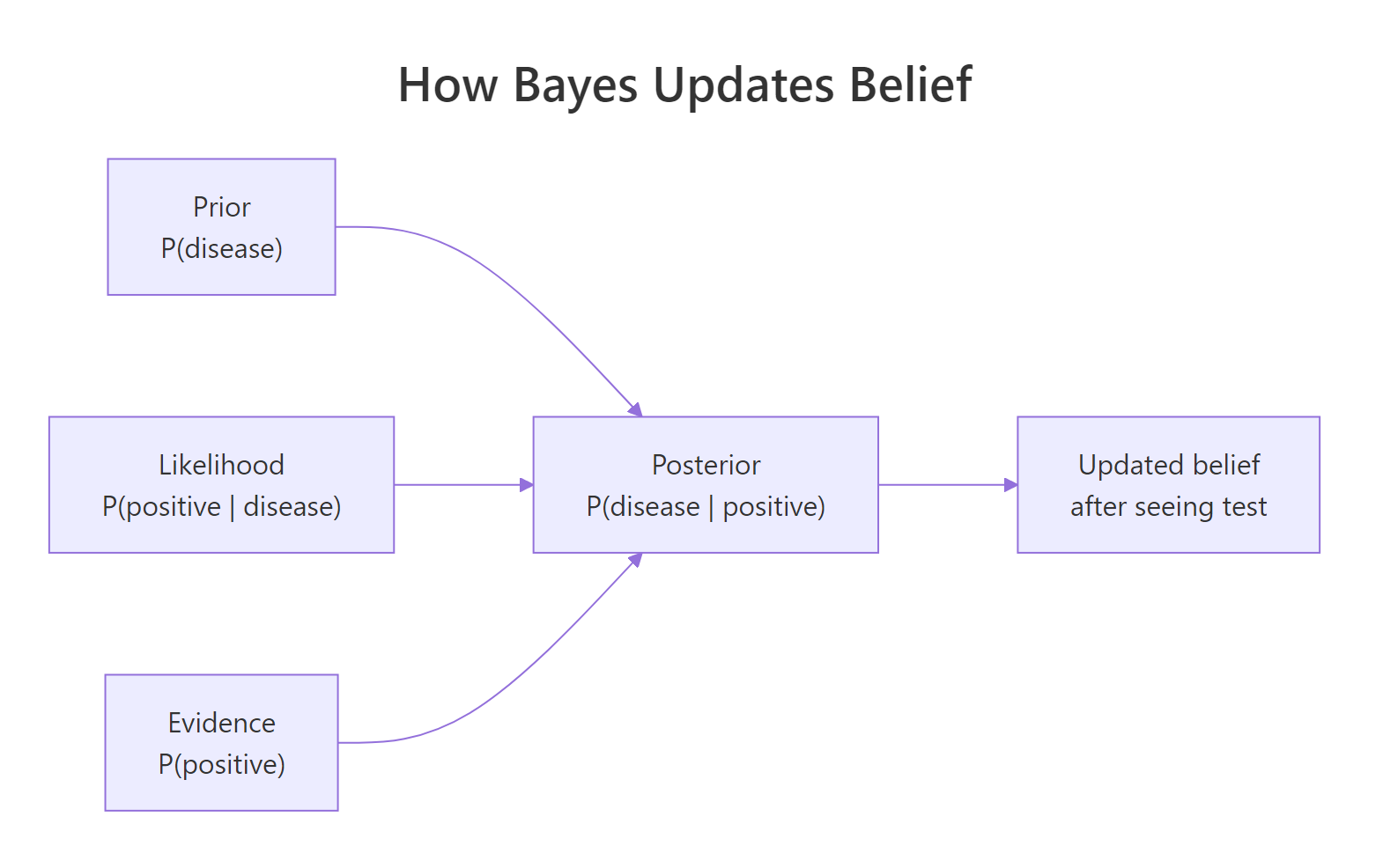
How Bayes combines prior, likelihood, and evidence into a posterior.

Figure 1: How Bayes combines prior, likelihood, and evidence into a posterior.

To see how PPV moves with disease prevalence, we hold sensitivity and specificity fixed at 99% and sweep the prior across a wide range.

RPlot PPV against disease prevalence

grid_df <- tibble( prevalence = seq(0.0001, 0.5, length.out = 200) ) |> mutate(ppv = bayes_pp(prevalence, sens = 0.99, spec = 0.99)) ggplot(grid_df, aes(x = prevalence, y = ppv)) + geom_line(color = "#1f77b4", size = 1) + scale_x_continuous(labels = scales::percent) + scale_y_continuous(labels = scales::percent) + labs(x = "Disease prevalence (prior)", y = "PPV (posterior on positive test)", title = "Even a 99% test gives low PPV at low prevalence") + theme_minimal()

The curve rises steeply from near zero at very low prevalence and approaches 100% only when prevalence is itself high. The same test is "99% accurate" in every scenario, yet its trustworthiness for any single positive result depends entirely on the prior. That single fact is the engine behind every misunderstanding about medical screening.

Key Insight

The same test gives different answers for different patients. A positive result is informative only relative to the patient's prior probability of the disease, which depends on age, exposure, and symptoms. The math is the same, the answer changes.

Try it: Use bayes_pp() to compute the PPV when prevalence is 5%, sensitivity is 95%, and specificity is 90%. Round to two decimal places.

RYour turn: PPV at 5% prevalence

# Try it: compute PPV for prev=0.05, sens=0.95, spec=0.90 ex_ppv <- # your code here round(ex_ppv, 2) #> Expected: 0.33

Click to reveal solution

RPPV at 5% prevalence solution

ex_ppv <- bayes_pp(prevalence = 0.05, sens = 0.95, spec = 0.90) round(ex_ppv, 2) #> [1] 0.33

Explanation: At 5% prevalence with 90% specificity, false positives still outnumber true positives nearly 2 to 1, so PPV lands at 33%, not 95%.

Why does a 99% accurate test return mostly false positives?

The answer is arithmetic, not statistics. When the disease is rare, the population of healthy people is enormous, and even a small false positive rate inside that huge group produces more false positives than the entire group of true positives combined.

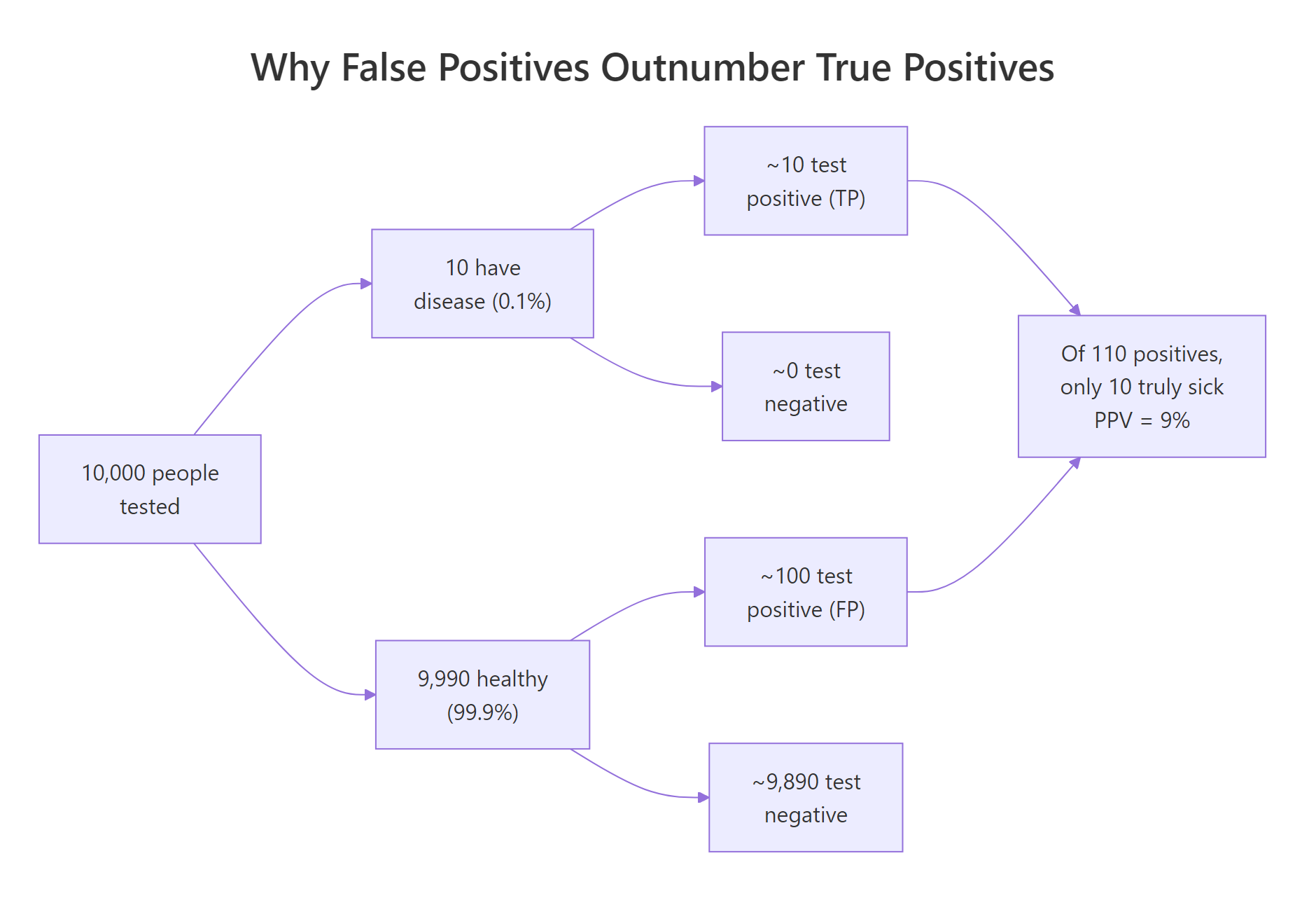
Why false positives can outnumber true positives when a disease is rare.

Figure 2: Why false positives can outnumber true positives when a disease is rare.

To make this concrete, let's simulate 10,000 people. We'll set prevalence to 0.1%, draw who has the disease, then assign each person a test result based on sensitivity (for the sick) and specificity (for the healthy). Counting outcomes turns the abstract probability into something you can see.

RSimulate 10,000 people and count test outcomes

set.seed(2026) n_total <- 10000 prevalence <- 0.001 sens <- 0.99 spec <- 0.99 # Disease status for each person (TRUE = has disease) has_disease <- runif(n_total) < prevalence # Test result: depends on whether they have it test_positive <- ifelse( has_disease, runif(n_total) < sens, runif(n_total) < (1 - spec) ) counts <- table(disease = has_disease, positive = test_positive) counts #> positive #> disease FALSE TRUE #> FALSE 9890 100 #> TRUE 0 10

The table tells the story directly. Among 9,990 healthy people, 100 still tested positive (false positives), while only 10 of the 10 sick people tested positive (true positives). Of the 110 positive results in total, just 10 are real, which gives an empirical PPV of 10 / 110, or about 9%.

RCompare empirical PPV to the analytical answer

empirical_ppv <- counts["TRUE", "TRUE"] / sum(counts[, "TRUE"]) analytical_ppv <- bayes_pp(prevalence, sens, spec) c(empirical = round(empirical_ppv, 4), analytical = round(analytical_ppv, 4)) #> empirical analytical #> 0.0909 0.0902

The two numbers agree to within sampling noise. The simulation is not telling us anything new beyond what the formula said; it is showing us the same result in counts of people, which our intuition handles better than ratios. The arithmetic of false positives is exactly Bayes' theorem in disguise.

Warning

Test "accuracy" is not PPV. A test marketed as "99% accurate" reports sensitivity and specificity, not the probability that a positive result reflects disease. Patients and journalists conflate the two. Always ask for prevalence before trusting any positive result.

Try it: Re-run the simulation with prevalence <- 0.10 (a 10% community prevalence rather than 0.1%) and observe how the empirical PPV changes.

RYour turn: simulate at higher prevalence

# Try it: change prevalence to 0.10 and recompute empirical PPV set.seed(2026) n_total <- 10000 prevalence <- # your value here sens <- 0.99 spec <- 0.99 has_disease <- runif(n_total) < prevalence test_positive <- ifelse(has_disease, runif(n_total) < sens, runif(n_total) < (1 - spec)) counts <- table(disease = has_disease, positive = test_positive) counts["TRUE", "TRUE"] / sum(counts[, "TRUE"]) #> Expected: ~0.92

Click to reveal solution

RSimulation at 10% prevalence solution

set.seed(2026) n_total <- 10000 prevalence <- 0.10 sens <- 0.99 spec <- 0.99 has_disease <- runif(n_total) < prevalence test_positive <- ifelse(has_disease, runif(n_total) < sens, runif(n_total) < (1 - spec)) counts <- table(disease = has_disease, positive = test_positive) round(counts["TRUE", "TRUE"] / sum(counts[, "TRUE"]), 3) #> [1] 0.916

Explanation: At 10% prevalence the sick group is 100 times larger than at 0.1%, so true positives now outnumber false positives by roughly 11 to 1. PPV jumps from 9% to over 90%, even though the test itself is unchanged.

How do sensitivity, specificity, and prevalence each shift PPV?

Three numbers drive PPV, and they pull in different directions. Sensitivity is $P(\text{positive} \mid \text{disease})$: how often the test catches a real case. Specificity is $P(\text{negative} \mid \text{no disease})$: how often the test correctly clears a healthy person. Prevalence is just $P(\text{disease})$, the prior. To see which lever matters most when the disease is rare, we hold prevalence at 0.1% and sweep specificity from 80% to 99.9%.

RSweep specificity, hold prevalence and sensitivity fixed

spec_grid <- seq(0.80, 0.999, length.out = 200) spec_df <- tibble( specificity = spec_grid, ppv = bayes_pp(prevalence = 0.001, sens = 0.99, spec = spec_grid) ) ggplot(spec_df, aes(x = specificity, y = ppv)) + geom_line(color = "#d62728", size = 1) + scale_x_continuous(labels = scales::percent) + scale_y_continuous(labels = scales::percent) + labs(x = "Specificity", y = "PPV at 0.1% prevalence", title = "Specificity dominates PPV at low prevalence") + theme_minimal()

The curve is almost flat below 95% specificity and explodes upward above 99.5%. Going from 95% to 99.9% specificity is the difference between a 2% PPV and a 50% PPV. Sensitivity helps you find disease, but specificity is what lets you trust a positive result when the disease is rare.

Tip

For rare conditions, optimise specificity first. A test that catches every case (high sensitivity) but flags 5% of healthy people (95% specificity) is nearly useless at low prevalence. Engineering the specificity from 95% to 99.5% has more impact than pushing sensitivity past 99%.

Try it: Wrap the formula in a tiny helper called ex_ppv() that takes prevalence, sensitivity, and specificity and returns PPV. Call it for prevalence 0.02, sens 0.98, spec 0.95.

RYour turn: write ex_ppv()

# Try it: implement ex_ppv() ex_ppv <- function(prev, sens, spec) { # your code here } round(ex_ppv(0.02, 0.98, 0.95), 3) #> Expected: 0.286

Click to reveal solution

Rex_ppv() solution

ex_ppv <- function(prev, sens, spec) { (sens * prev) / (sens * prev + (1 - spec) * (1 - prev)) } round(ex_ppv(0.02, 0.98, 0.95), 3) #> [1] 0.286

Explanation: At 2% prevalence with 95% specificity, only 29% of positives are real. The function reuses the same Bayes formula as bayes_pp() with renamed arguments.

What changes when you test twice?

A second positive test pushes the posterior much higher than a single test, but the math is not "99% accurate twice equals 99.99% accurate." Each test updates the prior with new evidence. Yesterday's posterior becomes today's prior. As long as the two tests are independent, you can apply Bayes twice in a row.

RSequential testing: apply Bayes twice

# After one positive test first_post <- bayes_pp(prevalence = 0.001, sens = 0.99, spec = 0.99) # That posterior is the prior for the second test second_post <- bayes_pp(prevalence = first_post, sens = 0.99, spec = 0.99) c(after_one_test = round(first_post, 3), after_two_tests = round(second_post, 3)) #> after_one_test after_two_tests #> 0.090 0.907

After one positive, PPV is 9%. After a second positive, PPV jumps to 91%. The same test, applied twice, took the result from "almost certainly a false alarm" to "very likely real." This is exactly how confirmatory testing works in clinics: the first test acts as a screen, and a second independent test is required before any diagnosis.

Note

Independence matters. If both tests share a failure mode, for example both rely on the same biomarker, they are not independent and Bayes will overstate the second posterior. Confirmatory tests should use a different mechanism, not a re-run of the same one.

Try it: What is the posterior probability of disease after three consecutive positive tests, all with sensitivity 99% and specificity 99%, starting from a prior of 0.001?

RYour turn: three sequential positives

# Try it: chain bayes_pp() three times prior <- 0.001 sens <- 0.99 spec <- 0.99 # your code here #> Expected: ~0.999

Click to reveal solution

RThree sequential positives solution

prior <- 0.001 sens <- 0.99 spec <- 0.99 p1 <- bayes_pp(prior, sens, spec) p2 <- bayes_pp(p1, sens, spec) p3 <- bayes_pp(p2, sens, spec) round(p3, 4) #> [1] 0.999

Explanation: Each application multiplies the odds in favour of the disease by the likelihood ratio. After three independent positives at 99% sensitivity and specificity, the posterior approaches certainty.

Where else does Bayes' theorem apply outside medicine?

The medical example is just one application of a general rule. Spam filters use Bayes to compute $P(\text{spam} \mid \text{words})$. Search engines rank pages by $P(\text{relevant} \mid \text{query})$. Machine learning classifiers, naive Bayes most directly, use the same arithmetic on text and image features. The events change, the formula does not.

RTiny Bayesian spam classifier

# Prior probabilities of spam vs ham p_spam <- 0.40 p_ham <- 0.60 # Word likelihoods given each class p_word_given_spam <- c(lottery = 0.30, meeting = 0.05) p_word_given_ham <- c(lottery = 0.01, meeting = 0.20) # A short email containing the word "lottery" word <- "lottery" posterior_spam <- (p_word_given_spam[word] * p_spam) / (p_word_given_spam[word] * p_spam + p_word_given_ham[word] * p_ham) round(unname(posterior_spam), 3) #> [1] 0.952

Given the prior that 40% of emails are spam, seeing the word "lottery" pushes the posterior to 95% spam. The same arithmetic that gave us PPV in medicine gives us the spam probability here. Whether the events are diseases, emails, or stock movements, Bayes is the bookkeeping rule for combining evidence with prior belief.

Key Insight

Bayes is general. Every probabilistic inference problem, from weather forecasts to recommendation systems, is some flavour of "update prior with likelihood." Once you see Bayes' theorem in one domain, the others become familiar.

Try it: Compute the posterior probability of spam given the word "meeting," using the same priors and likelihoods.

RYour turn: posterior for the word 'meeting'

# Try it: posterior P(spam | "meeting") p_spam <- 0.40 p_ham <- 0.60 p_word_given_spam <- c(lottery = 0.30, meeting = 0.05) p_word_given_ham <- c(lottery = 0.01, meeting = 0.20) # your code here #> Expected: ~0.143

Click to reveal solution

RPosterior for 'meeting' solution

word <- "meeting" posterior_spam <- (p_word_given_spam[word] * p_spam) / (p_word_given_spam[word] * p_spam + p_word_given_ham[word] * p_ham) round(unname(posterior_spam), 3) #> [1] 0.143

Explanation: "Meeting" is much more common in ham than spam, so seeing it lowers the posterior to about 14%, well below the 40% prior. The same formula gives different answers because the likelihoods flip.

Practice Exercises

These three exercises combine the ideas from earlier sections. Use distinct variable names like my_data and my_result so you don't overwrite the tutorial's variables in the same notebook session.

Exercise 1: COVID-style screening test

A community has 2% prevalence of an infection. The available test is 95% sensitive and 98% specific. Compute the PPV of a single positive test. Then find the lowest specificity that pushes PPV above 90% at the same prevalence and sensitivity.

RExercise 1: PPV and the specificity needed for PPV > 0.90

# Hint: bayes_pp() works element-wise on a vector of specificities # Write your code below:

Click to reveal solution

RExercise 1 solution

my_ppv <- bayes_pp(prevalence = 0.02, sens = 0.95, spec = 0.98) round(my_ppv, 3) #> [1] 0.492 spec_grid <- seq(0.95, 0.9999, length.out = 1000) my_curve <- bayes_pp(prevalence = 0.02, sens = 0.95, spec = spec_grid) my_required <- spec_grid[which(my_curve > 0.90)[1]] round(my_required, 4) #> [1] 0.9954

Explanation: At 98% specificity the PPV is only 49%. Pushing specificity to 99.54% raises PPV above 90%. Specificity is the dominant lever when prevalence is low.

Exercise 2: Two independent tests on a population

Simulate 50,000 people with 1% disease prevalence. Each person takes two independent tests, both with sensitivity 95% and specificity 97%. For each scenario below, compute the empirical PPV from the simulation and compare to Bayes:

(a) one positive test, (b) two consecutive positive tests, (c) one positive followed by one negative.

RExercise 2: Two-test simulation

# Hint: build two test_result vectors, then index combinations of TRUE/FALSE # Write your code below:

Click to reveal solution

RExercise 2 solution

set.seed(42) n <- 50000 prev <- 0.01 sens <- 0.95 spec <- 0.97 my_disease <- runif(n) < prev my_test1 <- ifelse(my_disease, runif(n) < sens, runif(n) < (1 - spec)) my_test2 <- ifelse(my_disease, runif(n) < sens, runif(n) < (1 - spec)) ppv_one <- mean(my_disease[my_test1]) ppv_both <- mean(my_disease[my_test1 & my_test2]) ppv_split <- mean(my_disease[my_test1 & !my_test2]) round(c(one_pos = ppv_one, both_pos = ppv_both, pos_then_neg = ppv_split), 3) #> one_pos both_pos pos_then_neg #> 0.246 0.910 0.013

Explanation: A single positive at 1% prevalence gives 25% PPV. Two consecutive positives push it to 91%. A positive followed by a negative collapses it to roughly 1%, near the prior. Each test moves the belief in proportion to its likelihood ratio.

Exercise 3: Naive Bayes email classifier

You have a vocabulary of five words: bonus, meeting, urgent, report, prize. Prior P(spam) = 0.4. Per-class word probabilities are below. Classify a 3-word email containing bonus, urgent, prize by computing the posterior probability of spam, treating the words as conditionally independent.

RExercise 3: 3-word naive Bayes classifier

# Hint: under conditional independence, multiply the word likelihoods p_spam <- 0.4 p_ham <- 0.6 p_w_spam <- c(bonus = 0.20, meeting = 0.05, urgent = 0.25, report = 0.05, prize = 0.30) p_w_ham <- c(bonus = 0.04, meeting = 0.20, urgent = 0.05, report = 0.15, prize = 0.01) email <- c("bonus", "urgent", "prize") # Write your code below:

Click to reveal solution

RExercise 3 solution

my_lik_spam <- prod(p_w_spam[email]) my_lik_ham <- prod(p_w_ham[email]) my_posterior_spam <- (my_lik_spam * p_spam) / (my_lik_spam * p_spam + my_lik_ham * p_ham) round(my_posterior_spam, 4) #> [1] 0.9991

Explanation: All three words are far more likely under spam than ham, so their likelihood ratios multiply, driving the posterior to over 99%. Naive Bayes scales this exact computation to thousands of words.

Putting It All Together

A clinic deploys two tests for a disease with 1% prevalence. Test A is 99% sensitive and 95% specific (a fast screen). Test B is 90% sensitive and 99.5% specific (a slow confirmatory test). We compute PPV after each test alone and after both tests positive.

RClinic scenario: two tests with different profiles

prev <- 0.01 # Test A: high sensitivity, lower specificity ppv_A <- bayes_pp(prevalence = prev, sens = 0.99, spec = 0.95) # Test B: lower sensitivity, very high specificity ppv_B <- bayes_pp(prevalence = prev, sens = 0.90, spec = 0.995) # Both A and B positive: A's posterior becomes B's prior ppv_AB <- bayes_pp(prevalence = ppv_A, sens = 0.90, spec = 0.995) scenario_summary <- tibble( scenario = c("A positive only", "B positive only", "A then B both positive"), ppv = c(ppv_A, ppv_B, ppv_AB) ) |> mutate(ppv = round(ppv, 3)) scenario_summary #> # A tibble: 3 x 2 #> scenario ppv #> <chr> <dbl> #> 1 A positive only 0.167 #> 2 B positive only 0.645 #> 3 A then B both positive 0.974

The summary makes the policy recommendation obvious. Test A by itself flags far too many false positives to act on (17% PPV), and Test B alone is decent (65%). But Test A followed by Test B both positive lifts the posterior above 97%. This is the rationale for two-stage screening: a sensitive screen catches everyone, then a specific confirmer rules out the false alarms.

Summary

Takeaway	What it means in code
Bayes = prior × likelihood / evidence	`bayes_pp(prev, sens, spec)` returns the posterior.
Low prevalence amplifies false positives	At 0.1% prevalence and 99% specificity, PPV is 9%, not 99%.
Specificity dominates PPV when disease is rare	Sweeping specificity reshapes PPV far more than sweeping sensitivity.
Sequential tests update the prior	Yesterday's posterior is today's prior; multiply likelihood ratios.
Same math powers spam, search, and ML	Naive Bayes is just Bayes' theorem on word features.

References

Gigerenzer, G. Reckoning with Risk: Learning to Live with Uncertainty. Penguin, 2002. The original framing of base rate fallacy in medical testing. Link
McElreath, R. Statistical Rethinking, 2nd Edition. CRC Press, 2020. Chapter 1: The Golem of Prague. Link
Wickham, H. and Grolemund, G. R for Data Science, 2nd Edition. O'Reilly, 2023. Chapters on simulation and dplyr summaries. Link
R Core Team. An Introduction to R. CRAN, 2024. Link
Diagnostic Testing and Bayes' Theorem. Medical Maths blog, 2024. R simulation walkthrough. Link

Continue Learning

Conjugate Priors in R explains the family of priors that make posteriors exact, no MCMC required, building directly on the belief-update intuition above.
Grid Approximation in R shows how to compute exact posteriors for any small model by evaluating Bayes on a grid of parameter values.
MCMC in R introduces Metropolis-Hastings, the algorithm that scales Bayes to high-dimensional models when the integrals stop being tractable.