Regression Tables in R: modelsummary vs stargazer vs gtsummary, Which to Use

A regression table turns a fitted model into a formatted grid of coefficients, standard errors, significance stars, and goodness-of-fit statistics that readers can scan at a glance. In R, three packages dominate this job: modelsummary, stargazer, and gtsummary. This tutorial shows you which one to pick and how to use each.

What makes a regression table publication-ready?

Anyone who has copy-pasted summary(lm(...)) into a Word document knows the feeling. The output is fine for the person who fit the model. It is unreadable for anyone else. A real regression table compresses the same fit into a compact grid where rows are coefficients and columns are either models or estimates. Here is the payoff. One line of R turns a bare lm() into a clean table your co-author will not complain about.

RLoad libraries and render your first table

library(modelsummary) library(tibble) # Fit a simple model on the built-in mtcars dataset fit_mpg <- lm(mpg ~ wt + hp, data = mtcars) # One line to produce a publication-ready table modelsummary(fit_mpg, output = "markdown") #> Model 1 #> (Intercept) 37.227 #> (1.599) #> wt -3.878 #> (0.633) #> hp -0.032 #> (0.009) #> Num.Obs. 32 #> R2 0.827 #> R2 Adj. 0.815 #> AIC 156.7 #> BIC 162.5 #> Log.Lik. -74.326

Notice what you got without any formatting work. Coefficients with standard errors stacked below, fit statistics at the bottom, clean column header. That is the baseline that every package in this tutorial aims for, with different defaults and different ways to customise it.

Try it: Fit a one-predictor model on mtcars (ex_fit1 <- lm(mpg ~ wt, data = mtcars)) and print it with modelsummary().

RYour turn: render a one-predictor fit

# Try it: fit and render a one-predictor model ex_fit1 <- # your code here modelsummary(ex_fit1, output = "markdown") #> Expected: a table with (Intercept), wt, Num.Obs., R2, AIC, BIC

Click to reveal solution

ROne-predictor solution

ex_fit1 <- lm(mpg ~ wt, data = mtcars) modelsummary(ex_fit1, output = "markdown") #> Model 1 #> (Intercept) 37.285 #> (1.878) #> wt -5.344 #> (0.559) #> Num.Obs. 32 #> R2 0.753

Explanation: modelsummary() accepts any fit object broom::tidy() understands. Single model, single column, same one-line call.

Key Insight

Publication tables differ from summary() in three ways. They show models side by side, let you pick which statistics appear, and export to the format you actually publish in, HTML, Word, LaTeX, or PDF.

How do modelsummary, stargazer, and gtsummary differ at a glance?

The three packages look similar on the surface, but they come from different traditions and optimise for different end products. modelsummary is a generalist built on top of the broom ecosystem. It supports more than a hundred model types out of the box and treats side-by-side comparison as the default. stargazer is the classic LaTeX-first package. It shaped what a "regression table in R" looks like for a decade and is still the default in many economics workflows. gtsummary comes from medical research. Its defaults assume categorical covariates, odds ratios, and clinical reporting conventions.

Here is a side-by-side feature matrix to anchor the rest of the tutorial.

Feature	modelsummary	stargazer	gtsummary
Default output	tinytable (HTML, LaTeX, Word)	Text, LaTeX, HTML	gt (HTML), flextable (Word)
Side-by-side models	Built-in	Built-in	Via `tbl_merge()`
Robust SEs	`vcov = "robust"`	Manual with `sandwich`	`add_vcov()`
Model types	100+ via broom/parameters	40+ hard-coded	Most broom-tidy models
Default style	Three-star significance	Journal-style dashes	Clinical, OR/HR columns
Active development	Yes (2026)	Maintenance mode	Yes (2026)

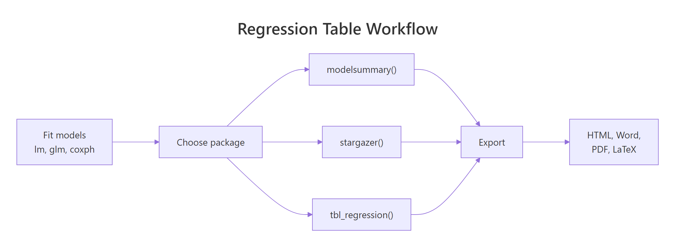
Workflow from fit to table to export with all three packages.

Figure 1: Every package follows the same three-step workflow: fit, table, export.

Warning

stargazer is in maintenance mode. The maintainer has publicly paused feature development. New model classes added to base R or tidymodels may not render cleanly. Your existing stargazer code will keep working, but new projects are better served by modelsummary or gtsummary.

Try it: Given the feature matrix above, name one scenario where each package is the best choice.

RYour turn: match package to scenario

# Try it: match each scenario to one package # A) Clinical trial paper with hazard ratios needed # B) Economics journal article, LaTeX workflow # C) Quick side-by-side of four lm() fits for a client # Answer A, B, C below (as strings): answer_a <- # your answer answer_b <- # your answer answer_c <- # your answer

Click to reveal solution

RScenario match solution

answer_a <- "gtsummary" # HR + clinical defaults answer_b <- "stargazer" # Classic LaTeX defaults, or modelsummary answer_c <- "modelsummary" # Fastest way to line up multiple fits c(answer_a, answer_b, answer_c) #> [1] "gtsummary" "stargazer" "modelsummary"

Explanation: gtsummary's built-in defaults for odds ratios, hazard ratios, and categorical reference rows save hours in clinical writing. stargazer and modelsummary both produce journal-ready LaTeX. For quick, multi-model comparisons with minimal code, modelsummary wins.

How do you build the same table with each package?

The fastest way to internalise the differences is to build the same table three ways. You fit the models once, then pass the same list to each package. Each call takes one line.

RFit three nested models on mtcars

# Fit three nested models predicting mpg fit1 <- lm(mpg ~ wt, data = mtcars) fit2 <- lm(mpg ~ wt + hp, data = mtcars) fit3 <- lm(mpg ~ wt + hp + cyl, data = mtcars) # Store in a named list so column headers match the names models <- list("Base" = fit1, "+HP" = fit2, "+Cyl" = fit3)

The named list is the key. Every package in this tutorial reads the names and uses them as column headers, so you get "Base", "+HP", "+Cyl" as column labels instead of "Model 1", "Model 2", "Model 3".

RSide-by-side with modelsummary

# modelsummary: the most direct call modelsummary(models, stars = TRUE, output = "markdown") #> Base +HP +Cyl #> (Intercept) 37.285 37.227 38.752 #> (1.878) (1.599) (1.787) #> wt -5.344*** -3.878*** -3.167*** #> (0.559) (0.633) (0.741) #> hp -0.032*** -0.018 #> (0.009) (0.012) #> cyl -0.942 #> (0.551) #> Num.Obs. 32 32 32 #> R2 0.753 0.827 0.843

Three models appear as three columns. The stars = TRUE argument adds significance stars with the standard thresholds ( = 0.001, = 0.01, = 0.05). Each coefficient sits above its standard error in parentheses.

RSide-by-side with stargazer

library(stargazer) # stargazer: same inputs, classic journal look stargazer(models, type = "text", column.labels = c("Base", "+HP", "+Cyl")) #> ====================================================== #> Dependent variable: #> ------------------------------------- #> mpg #> Base +HP +Cyl #> (1) (2) (3) #> ------------------------------------------------------ #> wt -5.344*** -3.878*** -3.167*** #> (0.559) (0.633) (0.741) #> hp -0.032*** -0.018 #> (0.009) (0.012) #> cyl -0.942* #> (0.551) #> Constant 37.285*** 37.227*** 38.752*** #> (1.878) (1.599) (1.787) #> ------------------------------------------------------ #> Observations 32 32 32 #> R-squared 0.753 0.827 0.843 #> ======================================================

Notice the differences. stargazer uses horizontal rules, puts the intercept as "Constant" at the bottom, and adds a "Dependent variable" banner across the top. This is the look of most economics and political science journals.

RSide-by-side with gtsummary

library(gtsummary) # gtsummary: one model at a time, merge for side-by-side t1 <- tbl_regression(fit1) t2 <- tbl_regression(fit2) t3 <- tbl_regression(fit3) tbl_merge(list(t1, t2, t3), tab_spanner = c("**Base**", "**+HP**", "**+Cyl**")) #> Characteristic Beta 95% CI p-value ... #> wt -5.3 (-6.5, -4.2) <0.001 #> hp -0.03 (-0.05, -0.01) <0.001 #> cyl -0.94 (-2.1, 0.19) 0.10

gtsummary takes a different route. It builds one table per model, then merges them with tbl_merge(). The default shows a 95% confidence interval instead of a standard error, and a p-value column, both clinical conventions.

Tip

Name your model list for clean column headers. modelsummary and gtsummary both read list names. list("Base" = fit1, "+HP" = fit2) produces headers "Base" and "+HP"; an unnamed list gives you "Model 1", "Model 2", etc.

Try it: Fit ex_fit_iris <- lm(Sepal.Length ~ Petal.Length + Petal.Width, data = iris) and build a stargazer text table for it.

RYour turn: stargazer on iris

# Try it: fit iris model and render with stargazer ex_fit_iris <- # your code here stargazer(# pass the fit and type = "text")

Click to reveal solution

Riris stargazer solution

ex_fit_iris <- lm(Sepal.Length ~ Petal.Length + Petal.Width, data = iris) stargazer(ex_fit_iris, type = "text") #> ========================================== #> Dependent variable: #> ---------------------------- #> Sepal.Length #> ------------------------------------------ #> Petal.Length 0.542*** #> (0.069) #> Petal.Width -0.320* #> (0.160) #> Constant 4.191*** #> (0.097) #> ------------------------------------------ #> Observations 150 #> R-squared 0.766

Explanation: type = "text" prints ASCII. Change to "latex" for a journal manuscript or "html" for a webpage.

How do you customize coefficients, standard errors, and fit stats?

Defaults get you a working table. Customisation gets you the table you actually want to ship. All three packages let you rename coefficients, reorder rows, select which fit statistics to show, and swap in robust standard errors. The syntax differs, but the concepts line up one to one.

Rmodelsummary customization

# Rename coefficients, reorder, pick fit stats, use robust SEs cm <- c("wt" = "Weight (1000 lbs)", "hp" = "Horsepower", "cyl" = "Cylinders", "(Intercept)" = "Intercept") modelsummary(models, coef_map = cm, gof_map = c("nobs", "r.squared", "aic"), stars = c("*" = 0.1, "**" = 0.05, "***" = 0.01), vcov = "robust", output = "markdown") #> Base +HP +Cyl #> Weight (1000 lbs) -5.344*** -3.878*** -3.167*** #> (0.587) (0.722) (0.824) #> Horsepower -0.032** -0.018 #> (0.011) (0.013) #> Cylinders -0.942 #> (0.642) #> Intercept 37.285*** 37.227*** 38.752*** #> (2.014) (1.833) (2.039) #> Num.Obs. 32 32 32 #> R2 0.753 0.827 0.843 #> AIC 166.0 156.7 156.0

Four arguments did the heavy lifting. coef_map renames and reorders rows. gof_map picks which fit statistics to show. stars redefines the thresholds. vcov = "robust" uses HC3 heteroskedasticity-robust standard errors, so the SEs in the output differ from the defaults above.

Rstargazer customization

# Rename labels, omit statistics, journal style stargazer(models, type = "text", covariate.labels = c("Weight (1000 lbs)", "Horsepower", "Cylinders"), omit.stat = c("ll", "ser", "f", "adj.rsq"), star.cutoffs = c(0.1, 0.05, 0.01)) #> ================================================================ #> Dependent variable: #> -------------------------------------------- #> mpg #> (1) (2) (3) #> ---------------------------------------------------------------- #> Weight (1000 lbs) -5.344*** -3.878*** -3.167*** #> Horsepower -0.032*** -0.018 #> Cylinders -0.942* #> Constant 37.285*** 37.227*** 38.752*** #> ---------------------------------------------------------------- #> Observations 32 32 32 #> R-squared 0.753 0.827 0.843 #> ================================================================

stargazer uses covariate.labels for renaming (in model order, not by name), omit.stat to drop fit statistics, and star.cutoffs to set thresholds. For robust SEs you compute the variance-covariance matrix yourself and pass a list of standard error vectors.

Rgtsummary customization

# Label variables, exponentiate coefficients, show p-values tbl_regression( fit3, label = list(wt ~ "Weight (1000 lbs)", hp ~ "Horsepower", cyl ~ "Cylinders"), estimate_fun = label_style_number(digits = 3) ) |> add_significance_stars() #> Characteristic Beta p-value #> Weight (1000 lbs) -3.167*** <0.001 #> Horsepower -0.018 0.148 #> Cylinders -0.942 0.097

gtsummary uses formula-based labels, a separate estimate_fun argument for numeric formatting, and add_significance_stars() to append stars to the estimate. It leans heavily on the pipe (|>) to chain these steps.

Note

Robust SEs are a one-liner in modelsummary. Pass vcov = "robust", "HC1", "HC3", or a function. In gtsummary, pipe through add_vcov(). In stargazer, compute the matrix with sandwich::vcovHC() and pass a list of SE vectors to the se argument, which takes more setup.

Try it: Rebuild the modelsummary(models) table with coef_map renaming wt to "Weight" and hp to "HP" only, leaving other rows untouched.

RYour turn: rename two coefficients

# Try it: rename two rows only ex_cm <- c(# fill in the mapping here) modelsummary(models, coef_map = ex_cm, output = "markdown") #> Expected: Weight and HP rows renamed; other rows still shown

Click to reveal solution

RRename solution

ex_cm <- c("wt" = "Weight", "hp" = "HP") modelsummary(models, coef_map = ex_cm, output = "markdown") #> Base +HP +Cyl #> Weight -5.344*** -3.878*** -3.167*** #> (0.559) (0.633) (0.741) #> HP -0.032*** -0.018 #> (0.009) (0.012)

Explanation: When coef_map is partial, only the mapped rows are renamed and reordered. Unmapped rows are dropped unless you include them in the mapping.

How do you export tables for PDF, Word, and HTML?

The piece that separates "fits in my notebook" from "lands in the published paper" is export. Each package is strongest in its home format. modelsummary is the most portable, gtsummary is the cleanest for Word, and stargazer is the fastest for LaTeX.

Target format	modelsummary	stargazer	gtsummary
HTML	`output = "file.html"`	`type = "html"`	`as_gt() \	> gt::gtsave()`
LaTeX	`output = "file.tex"`	`type = "latex"`	`as_kable_extra()`
Word (.docx)	`output = "file.docx"`	Via HTML + copy-paste	`as_flex_table()`
Markdown	`output = "markdown"`	`type = "text"`	`as_kable()`
Quarto / Rmd	Auto-detects	Needs `results = "asis"`	Auto-detects

Rmodelsummary direct export

# Write directly to a file, format inferred from extension modelsummary(models, output = "table.md") # You can also get a string back tab_str <- modelsummary(models, output = "markdown") class(tab_str) #> [1] "knitr_kable" "character"

modelsummary picks the format from the file extension. .docx triggers the flextable backend, .tex triggers LaTeX, .html triggers tinytable's HTML, and .md emits knitr's markdown kable.

Rgtsummary to Word and HTML

# Build once, convert to different backends t <- tbl_regression(fit3) # Convert to flextable for Word flex <- t |> as_flex_table() class(flex) #> [1] "flextable" # Convert to gt for HTML gt_obj <- t |> as_gt() class(gt_obj) #> [1] "gt_tbl" "list"

gtsummary separates table content from the rendering backend. You build the table once, then convert to gt for HTML (which supports CSS styling) or flextable for Word (which preserves tables cleanly in .docx).

Tip

In a Quarto or R Markdown document, skip the output argument. modelsummary() inspects the rendering target (HTML, PDF, or Word) and picks a sensible default. Hard-coding output = "html" breaks the LaTeX build.

Try it: Export the models list to a markdown string and store it in ex_md.

RYour turn: capture markdown output

# Try it: capture a table as a string ex_md <- # your call here cat(ex_md) #> Expected: markdown table with the three models

Click to reveal solution

RMarkdown capture solution

ex_md <- modelsummary(models, output = "markdown") class(ex_md) #> [1] "knitr_kable" "character" cat(ex_md) #> | | Base | +HP | +Cyl | #> |:------------------|:--------|:--------|:--------| #> | (Intercept) | 37.285 | 37.227 | 38.752 |

Explanation: output = "markdown" returns the table as a character vector you can paste into a document or log to a file.

Which package should you choose?

Here is the decision framework. Start from your output format and the conventions of your field, not from which package you saw first.

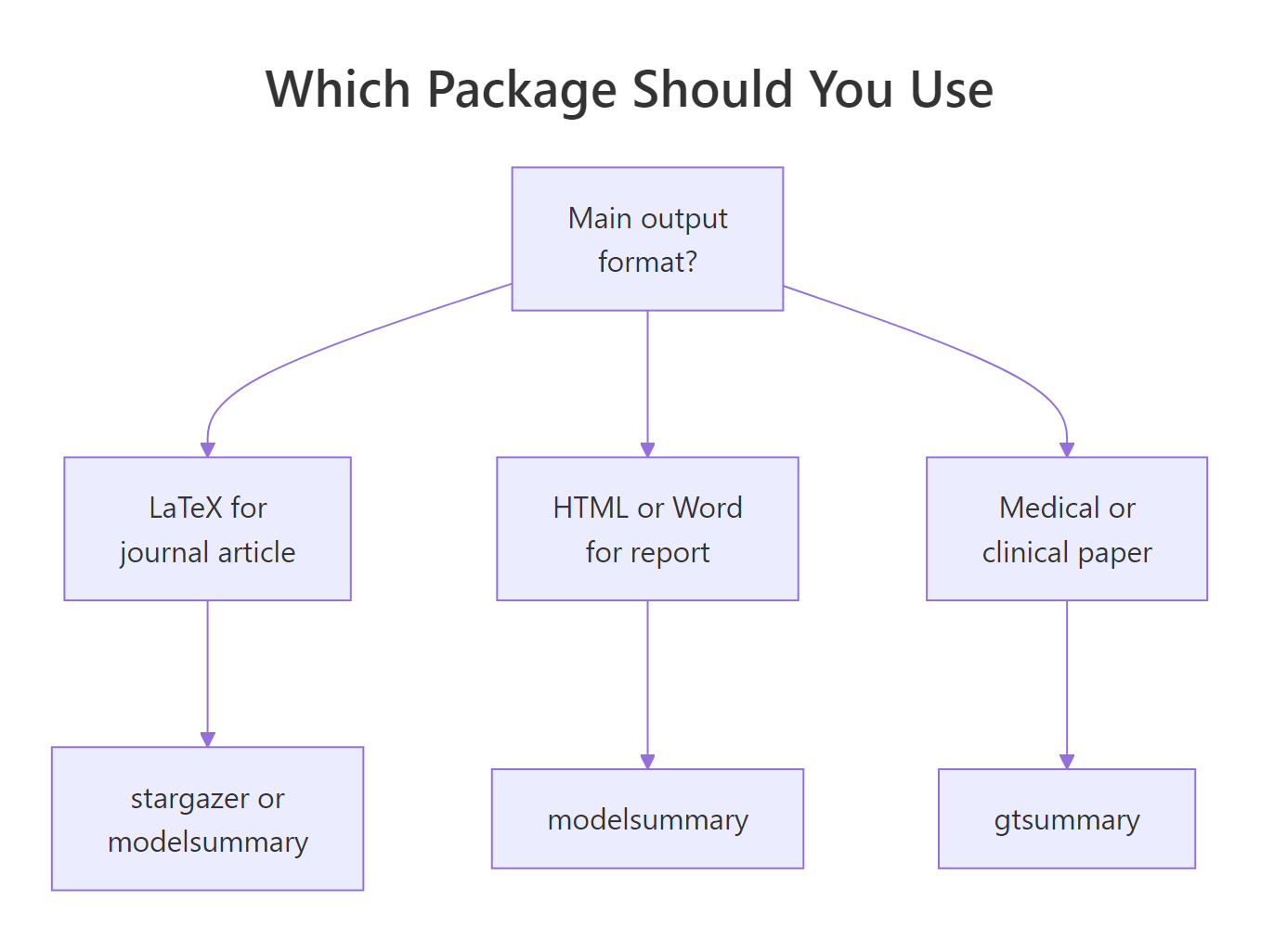
Decision tree for picking a regression table package based on output format.

Figure 2: A quick way to pick based on your output format.

The shortlist by use case:

LaTeX for an economics or finance journal: use modelsummary or stargazer. Both produce journal-compatible LaTeX. stargazer wins on default style, modelsummary wins on active development and model coverage.
Word or HTML for a client report: use modelsummary with output = "file.docx". Single call, portable, round-trips in Microsoft Word without manual fixes.
Clinical or medical paper: use gtsummary. The defaults assume odds ratios, categorical reference rows, and p-values, which match clinical reporting conventions (CONSORT, STROBE).
Comparing many models side by side: use modelsummary. gof_map, coef_map, and the named list interface scale cleanly to six or eight columns.
You need a model class stargazer does not support: use modelsummary. Any object with a broom::tidy() method works, including fixest, lme4, brms, survival, and many more.

Key Insight

If you learn only one, make it modelsummary. It is the most generalist and future-proof of the three. Reach for gtsummary when you publish medical research. Keep using stargazer only if you already have a working pipeline; it is in maintenance mode and new R model classes may not render cleanly.

Try it: For a fit from coxph(Surv(time, status) ~ age + sex), which package gives publication-ready output with the least code?

RYour turn: pick a package for Cox regression

# Try it: for Cox regression output, which single-word answer? # Hazard ratios, medical journal ex_choice <- # your answer ex_choice #> Expected: "gtsummary"

Click to reveal solution

RCox choice solution

ex_choice <- "gtsummary" ex_choice #> [1] "gtsummary"

Explanation: gtsummary recognises coxph objects automatically and exponentiates coefficients into hazard ratios by default. The table header says "HR" and reference rows appear for categorical covariates without extra configuration.

Practice Exercises

Exercise 1: Three-model comparison with custom labels

Using mtcars, fit three nested models predicting mpg, store them in a named list called my_models, and build a modelsummary table with coefficient labels renamed, three significance stars, and nobs plus aic as the only goodness-of-fit rows.

RExercise 1 starter

# Exercise: build a labelled three-model table # Fit three nested models (add one predictor per model) # Store as named list: my_models <- list("M1" = ..., "M2" = ..., "M3" = ...) # Call modelsummary with coef_map and gof_map my_models <- # your code my_cm <- # your rename map modelsummary(# your call)

Click to reveal solution

RExercise 1 solution

m1 <- lm(mpg ~ wt, data = mtcars) m2 <- lm(mpg ~ wt + hp, data = mtcars) m3 <- lm(mpg ~ wt + hp + cyl, data = mtcars) my_models <- list("M1" = m1, "M2" = m2, "M3" = m3) my_cm <- c("wt" = "Weight", "hp" = "Horsepower", "cyl" = "Cylinders", "(Intercept)" = "Intercept") modelsummary(my_models, coef_map = my_cm, gof_map = c("nobs", "aic"), stars = TRUE, output = "markdown") #> M1 M2 M3 #> Weight -5.344*** -3.878*** -3.167*** #> (0.559) (0.633) (0.741) #> Horsepower -0.032*** -0.018 #> (0.009) (0.012) #> Cylinders -0.942 #> (0.551) #> Intercept 37.285*** 37.227*** 38.752*** #> (1.878) (1.599) (1.787) #> Num.Obs. 32 32 32 #> AIC 166.0 156.7 156.0

Explanation: The named list gives you named columns. coef_map provides rename plus reorder; gof_map selects which fit rows appear.

Exercise 2: Replicate a stargazer table with modelsummary

Given this stargazer call, reproduce the same table with modelsummary.

RExercise 2 prompt

# Stargazer target: stargazer(fit3, type = "text", covariate.labels = c("Weight", "Horsepower", "Cylinders"), dep.var.labels = "Miles per gallon", omit.stat = c("ll", "ser", "f", "adj.rsq")) # Your job: same visual content with modelsummary

Click to reveal solution

RExercise 2 solution

rep_cm <- c("wt" = "Weight", "hp" = "Horsepower", "cyl" = "Cylinders", "(Intercept)" = "Intercept") modelsummary(list("Miles per gallon" = fit3), coef_map = rep_cm, gof_map = c("nobs", "r.squared"), stars = TRUE, output = "markdown") #> Miles per gallon #> Weight -3.167*** #> (0.741) #> Horsepower -0.018 #> (0.012) #> Cylinders -0.942 #> (0.551) #> Intercept 38.752*** #> (1.787) #> Num.Obs. 32 #> R2 0.843

Explanation: covariate.labels becomes coef_map. dep.var.labels becomes the list name. omit.stat becomes gof_map with only the stats you want to keep.

Exercise 3: Export a gtsummary logistic regression to Word and markdown

Fit a logistic regression predicting am (auto vs. manual transmission) from mpg and hp using glm(). Build a gtsummary table and convert it once to flextable (for Word) and once to as_kable() (for markdown).

RExercise 3 starter

# Exercise: gtsummary logistic regression, two exports my_log <- # fit the logistic regression my_tbl <- tbl_regression(# your args, exponentiate TRUE for OR) my_flex <- # convert to flextable my_kbl <- # convert to markdown

Click to reveal solution

RExercise 3 solution

my_log <- glm(am ~ mpg + hp, data = mtcars, family = binomial) my_tbl <- tbl_regression(my_log, exponentiate = TRUE) my_flex <- my_tbl |> as_flex_table() class(my_flex) #> [1] "flextable" my_kbl <- my_tbl |> as_kable() class(my_kbl) #> [1] "knitr_kable" "character"

Explanation: exponentiate = TRUE turns log odds into odds ratios. The header switches from "Beta" to "OR" automatically. The same table object converts to flextable for Word or kable for markdown without refitting.

Complete Example

Here is the end-to-end workflow most analysts run once per paper: fit the models, customise, add robust SEs, and export. The output is a self-contained HTML file you can email or attach to a pull request.

REnd-to-end regression reporting workflow

library(modelsummary) # 1. Fit the models base <- lm(mpg ~ wt, data = mtcars) plus_hp <- lm(mpg ~ wt + hp, data = mtcars) plus_cyl <- lm(mpg ~ wt + hp + cyl, data = mtcars) final_models <- list("Base" = base, "+ Horsepower" = plus_hp, "+ Cylinders" = plus_cyl) # 2. Define labels and goodness-of-fit selection final_cm <- c("wt" = "Weight (1000 lbs)", "hp" = "Horsepower", "cyl" = "Cylinders", "(Intercept)" = "Intercept") # 3. Render with robust SEs, three stars, clean fit stats modelsummary(final_models, coef_map = final_cm, gof_map = c("nobs", "r.squared", "adj.r.squared", "aic"), stars = c("*" = 0.1, "**" = 0.05, "***" = 0.01), vcov = "robust", title = "Fuel economy predictors (robust SEs, HC3)", notes = "Data: mtcars. HC3 robust standard errors in parentheses.", output = "markdown") #> Fuel economy predictors (robust SEs, HC3) #> Base + Horsepower + Cylinders #> Weight (1000 lbs) -5.344*** -3.878*** -3.167*** #> (0.587) (0.722) (0.824) #> Horsepower -0.032** -0.018 #> (0.011) (0.013) #> Cylinders -0.942 #> (0.642) #> Intercept 37.285*** 37.227*** 38.752*** #> (2.014) (1.833) (2.039) #> Num.Obs. 32 32 32 #> R2 0.753 0.827 0.843 #> R2 Adj. 0.745 0.815 0.826 #> AIC 166.0 156.7 156.0 #> Data: mtcars. HC3 robust standard errors in parentheses.

Change output = "markdown" to "table.html", "table.docx", or "table.tex" and you have the same table in your publication format of choice. No reshaping, no copy-paste into Excel.

Summary

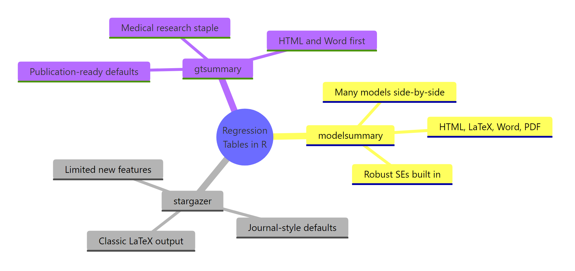
Overview of the three packages and their strongest use cases.

Figure 3: The three packages and their strongest use cases.

Package	Pick when...	Skip when...
modelsummary	You want one tool for every workflow, many model types, active development	Your field mandates gtsummary defaults
stargazer	Your existing LaTeX pipeline uses it and works	You need a model type added after 2020
gtsummary	You write clinical or medical papers, need OR/HR defaults	You need LaTeX-first journal output

Key takeaways:

All three accept the same fit objects, so switching packages never means refitting models.
Named lists give you clean column headers in modelsummary and gtsummary.
Robust SEs are one argument in modelsummary (vcov = "robust"), one pipe in gtsummary (add_vcov()), and manual work in stargazer.
modelsummary is the generalist choice in 2026; gtsummary is best for medical publishing; stargazer remains usable but is in maintenance mode.

References

Arel-Bundock, V. (2022). modelsummary: Data and Model Summaries in R. Journal of Statistical Software, 103(1). Link
modelsummary documentation. Link
Hlavac, M. (2022). stargazer: Well-Formatted Regression and Summary Statistics Tables. CRAN package version 5.2.3. Link
Sjoberg, D., Whiting, K., Curry, M., Lavery, J., Larmarange, J. (2021). Reproducible Summary Tables with the gtsummary Package. The R Journal, 13(1). Link
gtsummary tbl_regression vignette. Link
Princeton Library, A Hands-on R Tutorial Using Stargazer. Link
Tilburg Science Hub, Generate Regression Tables in R with the modelsummary Package. Link
tinytable documentation (modelsummary's default backend since v2.0). Link

Continue Learning

Linear Regression: fit the lm() models this tutorial formats.
Logistic Regression with R: the glm() binary-outcome models that gtsummary exponentiates into odds ratios.
Linear Regression Assumptions in R: verify your fits before you report them in a table.

Regression Tables in R: modelsummary vs stargazer vs gtsummary, Which to Use

What makes a regression table publication-ready?

How do modelsummary, stargazer, and gtsummary differ at a glance?

How do you build the same table with each package?

How do you customize coefficients, standard errors, and fit stats?

How do you export tables for PDF, Word, and HTML?

Which package should you choose?

Practice Exercises

Exercise 1: Three-model comparison with custom labels

Exercise 2: Replicate a stargazer table with modelsummary

Exercise 3: Export a gtsummary logistic regression to Word and markdown

Complete Example

Summary

References

Continue Learning

Related Tutorials