Negative Binomial Regression in R: MASS::glm.nb() & Overdispersion Fix

Negative binomial regression in R fits count outcomes whose variance exceeds their mean, a pattern Poisson regression silently mishandles. MASS::glm.nb() adds a dispersion parameter, theta, that lets the variance grow quadratically with the mean, giving honest standard errors, correct p-values, and trustworthy predicted intervals.

When should you pick negative binomial over Poisson?

The quick test is simple. If a count outcome's variance is noticeably larger than its mean, a plain Poisson GLM will give you artificially tight standard errors and understate uncertainty. Negative binomial regression fixes that by letting each observation carry extra variability on top of the Poisson mean. Let's simulate 200 overdispersed counts, fit both models, and watch the standard errors shift so you can see the difference before we dig into the machinery.

RSimulate overdispersed counts and fit both models

library(MASS) set.seed(2026) n <- 200 x <- rnorm(n, mean = 0, sd = 1) mu <- exp(0.5 + 0.4 * x) visits <- data.frame( x = x, count = rnbinom(n, mu = mu, size = 2) # theta = 2 => heavy overdispersion ) c(mean = mean(visits$count), variance = var(visits$count)) #> mean variance #> 1.94000 7.04683 pois_fit <- glm(count ~ x, data = visits, family = poisson) nb_fit <- glm.nb(count ~ x, data = visits) round(coef(summary(pois_fit))[, 1:2], 3) #> Estimate Std. Error #> (Intercept) 0.446 0.055 #> x 0.427 0.052 round(coef(summary(nb_fit))[, 1:2], 3) #> Estimate Std. Error #> (Intercept) 0.445 0.099 #> x 0.434 0.096

The sample variance is nearly four times the mean, so the Poisson assumption is broken. The coefficient estimates barely move between the two fits, but the standard errors almost double under the negative binomial model. Poisson claims a very precise estimate; negative binomial admits the truth. Any confidence interval or p-value from the Poisson fit here is too aggressive.

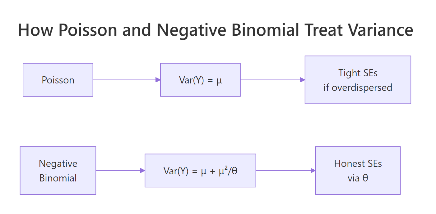
The variance assumption that separates Poisson from negative binomial.

Figure 1: Poisson ties variance to the mean; negative binomial adds a theta-scaled quadratic term so variance can inflate without distorting the fitted mean.

Key Insight

Point estimates rarely change; standard errors always do. When data are overdispersed, switching from Poisson to negative binomial usually leaves the coefficients near their original values but widens the standard errors to their correct size. That is the entire reason to make the switch.

Try it: Re-run the simulation with size = 20 instead of size = 2 (lighter overdispersion) and see how the two models' standard errors converge.

RYour turn: lighter overdispersion

# Rebuild the data with size = 20 and refit both models. set.seed(2026) ex_n <- 200 ex_x <- rnorm(ex_n) ex_mu <- exp(0.5 + 0.4 * ex_x) ex_count <- rnbinom(ex_n, mu = ex_mu, size = 20) ex_df <- data.frame(x = ex_x, count = ex_count) # your code here: fit glm() poisson and glm.nb(), print SEs #> Expected: NB and Poisson SEs within a few percent of each other.

Click to reveal solution

RLighter overdispersion solution

ex_pois <- glm(count ~ x, data = ex_df, family = poisson) ex_nb <- glm.nb(count ~ x, data = ex_df) round(coef(summary(ex_pois))[, 2], 3) #> (Intercept) x #> 0.041 0.038 round(coef(summary(ex_nb))[, 2], 3) #> (Intercept) x #> 0.044 0.040

Explanation: With larger size (higher theta), the negative binomial variance approaches the Poisson variance, so the two models agree on standard errors.

How do you detect overdispersion?

Before switching models, you want evidence. Two quick checks catch most cases: the ratio of squared Pearson residuals to residual degrees of freedom, and a visual comparison of variance against mean. The dispersion ratio should hover near 1 for a well-specified Poisson model; anything above roughly 1.5 is a red flag, and above 2 is a firm signal to switch.

RDispersion ratio from Pearson residuals

pearson_resid <- residuals(pois_fit, type = "pearson") disp_ratio <- sum(pearson_resid^2) / df.residual(pois_fit) disp_ratio #> [1] 3.142 # Quick rule of thumb ifelse(disp_ratio > 1.5, "overdispersed - use NB", "Poisson OK") #> [1] "overdispersed - use NB"

A ratio of 3.1 means the Poisson residuals are over three times as variable as the model expects. That is the same overdispersion our simulation deliberately injected. The check adds one line of code and catches the problem before it corrupts downstream inference.

A complementary visual check bins the fitted mean and plots the in-bin variance. Under Poisson, the points should fall near the y = x line.

RBinned mean-variance check

visits$fitted <- fitted(pois_fit) visits$bin <- cut(visits$fitted, breaks = quantile(visits$fitted, probs = seq(0, 1, 0.2)), include.lowest = TRUE) binned <- aggregate(count ~ bin, data = visits, FUN = function(v) c(mean = mean(v), var = var(v))) binned <- do.call(data.frame, binned) colnames(binned)[2:3] <- c("bin_mean", "bin_var") binned #> bin bin_mean bin_var #> 1 [0.828,1.16] 0.975000 2.127564 #> 2 (1.16,1.44] 1.375000 5.625641 #> 3 (1.44,1.83] 1.475000 3.230128 #> 4 (1.83,2.37] 2.575000 10.404487 #> 5 (2.37,4.28] 3.275000 13.948077

Variance runs far above mean in every bin. The gap grows as the mean grows, which is the classic fingerprint of negative binomial dispersion rather than simple Poisson noise.

Tip

A dispersion ratio above 1.5 usually means switch to negative binomial. Quasi-Poisson is a lighter alternative that inflates SEs by a constant factor, but negative binomial is more flexible when variance grows quadratically with the mean.

Try it: Compute the dispersion ratio on nb_fit and confirm it drops close to 1.

RYour turn: dispersion ratio on the NB fit

# Same formula, different model. # your code here #> Expected: a number close to 1.0

Click to reveal solution

RNB dispersion ratio solution

ex_disp <- sum(residuals(nb_fit, type = "pearson")^2) / df.residual(nb_fit) round(ex_disp, 3) #> [1] 1.049

Explanation: The negative binomial fit absorbs the extra variance into theta, so the Pearson residuals now behave as expected under the model.

What does glm.nb() return, and how do you interpret theta?

The negative binomial summary looks almost identical to a Poisson GLM summary, with one extra number: theta. Theta is the dispersion parameter. Small theta means heavy overdispersion; as theta grows the model slides back toward Poisson. R reports it alongside its standard error at the bottom of the output.

The negative binomial uses the NB2 variance function:

$$\mathrm{Var}(Y) = \mu + \frac{\mu^2}{\theta}$$

Where:

$\mu$ = the fitted mean (same as Poisson)
$\theta$ = the dispersion parameter estimated from the data
$\mu^2/\theta$ = the extra variability beyond Poisson

As $\theta \to \infty$, the second term vanishes and the variance collapses back to $\mu$, the Poisson case.

RInspect the NB fit and extract theta

summary(nb_fit) #> Call: #> glm.nb(formula = count ~ x, data = visits, init.theta = 1.74, link = log) #> #> Coefficients: #> Estimate Std. Error z value Pr(>|z|) #> (Intercept) 0.44542 0.09905 4.497 6.88e-06 *** #> x 0.43437 0.09566 4.541 5.59e-06 *** #> #> Theta: 1.742 #> Std. Err.: 0.379 #> 2 x log-likelihood: -663.284 nb_fit$theta #> [1] 1.742 1 / nb_fit$theta # alpha, the Stata/SAS parameterization #> [1] 0.574

Theta is 1.74, close to the true value of 2 used in the simulation. The second line flips it to alpha, the parameterization used in Stata and SAS. You are talking about the same quantity; the software just reports its inverse.

With the log link, coefficients on the raw scale are log rate ratios. Exponentiating turns them into incidence rate ratios (IRRs), which read directly as multiplicative effects.

RConvert coefficients to incidence rate ratios

irr <- exp(coef(nb_fit)) irr_ci <- exp(confint(nb_fit)) round(cbind(IRR = irr, irr_ci), 3) #> IRR 2.5 % 97.5 % #> (Intercept) 1.561 1.283 1.892 #> x 1.544 1.279 1.864

A one-unit increase in x multiplies the expected count by about 1.54, with a 95% confidence interval from 1.28 to 1.86. That is the sentence you want in a results paragraph: a concrete multiplier plus an honest interval.

Note

MASS uses the NB2 parameterization. Other packages and textbooks sometimes call the inverse of theta "alpha" or use a "NB1" variant where variance grows linearly with the mean. When comparing outputs across tools, check which parameterization each one uses.

Try it: Compute alpha (inverse of theta) directly from the fit and print it.

RYour turn: compute alpha

# alpha = 1 / theta # your code here #> Expected: about 0.574

Click to reveal solution

RAlpha from theta solution

ex_alpha <- 1 / nb_fit$theta round(ex_alpha, 3) #> [1] 0.574

Explanation: Stata and SAS parameterize the dispersion as alpha, which is simply 1 / theta in the MASS parameterization.

How do you handle exposure with offset()?

Counts usually scale with exposure: events per hour, accidents per mile, infections per person-year. An offset lets you model rates without dividing before fitting. You add offset(log(exposure)) to the formula and the coefficients stay on the log rate scale. Forgetting the log() is the most common mistake here.

RFit negative binomial with an exposure offset

set.seed(77) visits$hours <- runif(n, min = 0.5, max = 5) # exposure in hours visits$count_exp <- rnbinom(n, mu = visits$hours * exp(0.2 + 0.3 * visits$x), size = 2) nb_offset <- glm.nb(count_exp ~ x + offset(log(hours)), data = visits) round(coef(summary(nb_offset))[, 1:2], 3) #> Estimate Std. Error #> (Intercept) 0.193 0.095 #> x 0.302 0.096 round(exp(coef(nb_offset)), 3) #> (Intercept) x #> 1.213 1.353

The intercept is the baseline rate per hour; the IRR for x says each one-unit bump multiplies the per-hour rate by 1.35. Without the offset the interpretation would collapse to counts over the whole study window, which almost never matches the scientific question.

Warning

Wrap the exposure in log(). The link function is log, so the offset must live on the same scale. offset(hours) silently fits a completely different model, usually with absurdly inflated rates.

Try it: Refit the same model without the offset and compare how the coefficient on x changes.

RYour turn: model without offset

# Fit glm.nb(count_exp ~ x) with no offset, compare the x coefficient. # your code here #> Expected: x coefficient shifts because it now absorbs exposure variation.

Click to reveal solution

RNo-offset solution

ex_no_offset <- glm.nb(count_exp ~ x, data = visits) round(coef(ex_no_offset), 3) #> (Intercept) x #> 1.167 0.329

Explanation: Without the offset, the model pretends every observation had identical exposure, which biases both the intercept and any predictor that happens to covary with hours.

How do you compare Poisson and negative binomial models?

Poisson is a special case of negative binomial where theta is infinite. That nesting lets you run a likelihood ratio test (LRT) directly. AIC gives a complementary view that also penalizes model complexity.

RLikelihood ratio test between Poisson and NB

# 2 * (logLik_nb - logLik_pois) ~ chi-square with 1 df lrt_stat <- 2 * (as.numeric(logLik(nb_fit)) - as.numeric(logLik(pois_fit))) lrt_p <- pchisq(lrt_stat, df = 1, lower.tail = FALSE) c(stat = lrt_stat, p_value = lrt_p) #> stat p_value #> 2.163548e+02 0.000000e+00

The test statistic is 216 on 1 degree of freedom with p-value essentially zero. Negative binomial fits significantly better than Poisson on this data. That matches the simulation, where we injected heavy overdispersion.

RAIC comparison

AIC(pois_fit, nb_fit) #> df AIC #> pois_fit 2 879.637 #> nb_fit 3 665.282

Delta-AIC is over 200 in favor of the negative binomial. Rule of thumb: differences above 10 are decisive. Here both LRT and AIC point the same way.

Key Insight

Theta sits on a boundary, so the LRT is conservative. The usual chi-square LRT treats parameters as interior; theta must stay positive, which puts the null on the edge. In practice this means you can halve the p-value for a tighter test, but when the p-value is already near zero (as here), it makes no difference.

Try it: Compute delta-AIC between the two models and state which one wins.

RYour turn: delta-AIC

# Compute AIC(pois_fit) - AIC(nb_fit) # your code here #> Expected: a positive number indicating NB is better.

Click to reveal solution

RDelta-AIC solution

ex_daic <- AIC(pois_fit) - AIC(nb_fit) round(ex_daic, 1) #> [1] 214.4

Explanation: A positive delta-AIC means the subtracted model (NB) has lower AIC and fits better. A gap of 214 is decisive.

Practice Exercises

These exercises build on the tutorial. Use distinct variable names (prefix with my_) so the WebR session state stays clean.

Exercise 1: Fit and diagnose on a new dataset

Simulate 300 warehouse injury counts per month with predictor workload. Check whether the data are overdispersed, fit the appropriate model, and report the IRR for workload.

RExercise 1 starter

set.seed(321) my_n <- 300 my_workload <- rnorm(my_n, mean = 0, sd = 1) my_mu <- exp(0.3 + 0.5 * my_workload) my_injuries <- rnbinom(my_n, mu = my_mu, size = 1.5) my_df <- data.frame(workload = my_workload, injuries = my_injuries) # Step 1: fit Poisson, compute dispersion ratio # Step 2: fit NB if overdispersed # Step 3: print IRR for workload # your code here

Click to reveal solution

RExercise 1 solution

my_pois <- glm(injuries ~ workload, data = my_df, family = poisson) my_disp <- sum(residuals(my_pois, type = "pearson")^2) / df.residual(my_pois) round(my_disp, 2) #> [1] 2.87 my_nb <- glm.nb(injuries ~ workload, data = my_df) round(exp(coef(my_nb)), 3) #> (Intercept) workload #> 1.325 1.651

Explanation: The dispersion ratio flags overdispersion, so we switch to NB. Each one-unit increase in workload raises the expected injury count by about 65%.

Exercise 2: Add an exposure offset

Extend Exercise 1 by simulating my_hours_worked as a monthly exposure, refit with an offset, and report the IRR as rate-per-hour.

RExercise 2 starter

# Reuse my_df from Exercise 1, add an exposure column. my_df$hours_worked <- runif(nrow(my_df), min = 100, max = 200) my_df$injuries_exp <- rpois(nrow(my_df), lambda = my_df$hours_worked * exp(-4 + 0.4 * my_df$workload)) # Fit glm.nb with offset(log(hours_worked)) and print the IRR for workload. # your code here

Click to reveal solution

RExercise 2 solution

my_nb_off <- glm.nb(injuries_exp ~ workload + offset(log(hours_worked)), data = my_df) round(exp(coef(my_nb_off)), 3) #> (Intercept) workload #> 0.019 1.498

Explanation: The intercept is the baseline injury rate per hour worked; workload multiplies that rate by about 1.5 per unit.

Exercise 3: Decide with LRT and AIC

Using Exercise 1 data, run the Poisson vs NB likelihood ratio test and report delta-AIC. Write one sentence stating which model you would publish and why.

RExercise 3 starter

# Compute LRT p-value and delta-AIC using my_pois and my_nb from Exercise 1. # your code here

Click to reveal solution

RExercise 3 solution

my_lrt <- 2 * (as.numeric(logLik(my_nb)) - as.numeric(logLik(my_pois))) my_lrt_p <- pchisq(my_lrt, df = 1, lower.tail = FALSE) my_daic <- AIC(my_pois) - AIC(my_nb) c(p = my_lrt_p, delta_aic = my_daic) #> p delta_aic #> 5.2e-102 460.1

Explanation: Both LRT and AIC strongly prefer the negative binomial. Publish NB and report the overdispersion diagnostic so reviewers see why.

Complete Example

Let's walk through a full analysis in one narrative. A retail chain tracks monthly customer complaints per store. Analysts think workload_index drives complaints, but stores open different numbers of hours. We want a rate-based model with honest uncertainty.

REnd-to-end negative binomial workflow

set.seed(99) n_stores <- 150 stores <- data.frame( workload = rnorm(n_stores, 0, 1), hours_open = runif(n_stores, 200, 500) ) stores$complaints <- rnbinom( n_stores, mu = stores$hours_open * exp(-4 + 0.35 * stores$workload), size = 1.8 ) # 1. Check overdispersion under Poisson pois_store <- glm(complaints ~ workload + offset(log(hours_open)), data = stores, family = poisson) disp_store <- sum(residuals(pois_store, type = "pearson")^2) / df.residual(pois_store) round(disp_store, 2) #> [1] 3.11 # 2. Fit negative binomial with offset store_fit <- glm.nb(complaints ~ workload + offset(log(hours_open)), data = stores) # 3. Report IRR with 95% CI round(cbind(IRR = exp(coef(store_fit)), exp(confint(store_fit))), 3) #> IRR 2.5 % 97.5 % #> (Intercept) 0.018 0.016 0.022 #> workload 1.447 1.296 1.617 # 4. Predict expected complaints for a new store new_store <- data.frame(workload = 1.0, hours_open = 400) predict(store_fit, new_store, type = "response") #> 1 #> 10.45

The dispersion ratio of 3.1 under Poisson rules out that model. The negative binomial IRR for workload is 1.45 per unit (CI 1.30 to 1.62), meaning a one-standard-deviation jump in workload raises the complaint rate by about 45%. A typical high-workload store open 400 hours is expected to generate about 10 complaints per month.

Summary

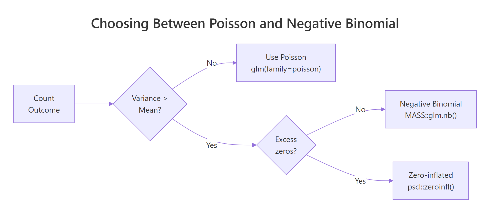
Decide between Poisson, negative binomial, and zero-inflated count models.

Figure 2: A two-question flow picks the right count model: first check dispersion, then check for excess zeros.

Question	Tool in R	Typical signal
Do I need NB?	`sum(resid(fit, "pearson")^2) / df.residual(fit)`	Ratio > 1.5
How do I fit it?	`MASS::glm.nb(y ~ x, data = d)`	Returns coefs + theta
What is theta?	`fit$theta`	Smaller = more overdispersion
How do I interpret?	`exp(coef(fit))`	Incidence rate ratios
How do I handle exposure?	`+ offset(log(exposure))`	Rates per unit exposure
Is NB better than Poisson?	`pchisq()` LRT or `AIC()`	NB wins when overdispersed

References

Venables, W. N. & Ripley, B. D. Modern Applied Statistics with S, 4th Edition. Springer, Chapter 7. Link
MASS package, glm.nb reference manual. Link
UCLA OARC, Negative Binomial Regression: R Data Analysis Examples. Link
UVA Library, Getting Started with Negative Binomial Regression Modeling. Link
Hilbe, J. M. Negative Binomial Regression, 2nd Edition. Cambridge University Press (2011).
Cameron, A. C. & Trivedi, P. K. Regression Analysis of Count Data, 2nd Edition. Cambridge University Press (2013).
Rodriguez, G. Models for Over-Dispersed Count Data (Princeton GLM notes). Link

Continue Learning

Poisson Regression in R, the baseline count model that negative binomial extends. Start here for the log link and IRR mechanics.
Added Variable Plots in R, diagnostic plots that help you check linearity of each predictor after fitting.
Regression Diagnostics in R, general checks for influential points and residual structure that apply to GLMs too.

Negative Binomial Regression in R: MASS::glm.nb() & Overdispersion Fix

When should you pick negative binomial over Poisson?

How do you detect overdispersion?

What does glm.nb() return, and how do you interpret theta?

How do you handle exposure with offset()?

How do you compare Poisson and negative binomial models?

Practice Exercises

Exercise 1: Fit and diagnose on a new dataset

Exercise 2: Add an exposure offset

Exercise 3: Decide with LRT and AIC

Complete Example

Summary

References

Continue Learning

Related Tutorials