Beta Regression in R: betareg Package for Proportions & Rates

Beta regression models continuous outcomes bounded between 0 and 1, such as proportions, percentages, and rates, using a beta distribution and link functions. The betareg package fits these models with a formula interface similar to lm().

When should you use beta regression instead of linear or logistic regression?

Proportions, yields, and rates often look like they should fit in a linear model, yet they refuse to cooperate. Predictions leak below 0 and above 1, variance shrinks near the edges, and residuals fan out. Beta regression solves this by modelling the response as a draw from a beta distribution, a flexible shape that lives strictly inside (0, 1). Here is the payoff on Prater's gasoline yield data.

RFit beta regression on GasolineYield

library(betareg) gy <- GasolineYield m1 <- betareg(yield ~ batch + temp, data = gy) summary(m1) #> Call: #> betareg(formula = yield ~ batch + temp, data = gy) #> #> Standardized weighted residuals 2: #> Min 1Q Median 3Q Max #> -2.8750 -0.8149 0.1601 0.8384 2.0483 #> #> Coefficients (mean model with logit link): #> Estimate Std. Error z value Pr(>|z|) #> (Intercept) -6.1595710 0.1823247 -33.783 < 2e-16 *** #> batch1 1.7277030 0.1012294 17.067 < 2e-16 *** #> batch2 1.3225456 0.1177780 11.229 < 2e-16 *** #> ... #> temp 0.0109669 0.0004126 26.577 < 2e-16 *** #> #> Phi coefficients (precision model with identity link): #> Estimate Std. Error z value Pr(>|z|) #> (phi) 440.28 110.02 4.002 6.29e-05 *** #> #> Type of estimator: ML (maximum likelihood) #> Log-likelihood: 84.8 on 12 Df #> Pseudo R-squared: 0.9617

The response yield is the fraction of crude oil converted to gasoline after distillation, a clean (0, 1) proportion. The summary has two blocks: the mean model with a logit link (the fraction itself) and a precision model that controls how tightly observations cluster around the mean. A pseudo R² of 0.96 tells you temperature and batch explain almost all of the variation in yield.

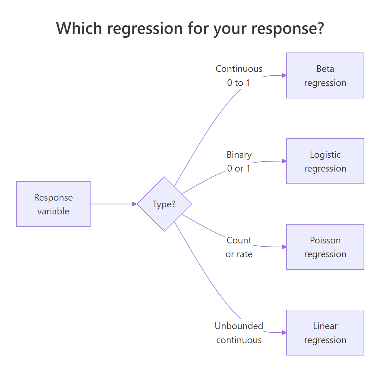
Decision flow for choosing between linear, logistic, and beta regression

Figure 1: A decision guide for choosing between linear, logistic, and beta regression based on the response variable.

Linear regression is the wrong tool here because it happily predicts a yield of 1.2 or −0.1 when extrapolating. Logistic regression is also wrong, even though it uses the same logit link, because it assumes the outcome is Bernoulli (a yes/no count out of trials), not a continuous fraction.

Key Insight

Beta regression replaces the Gaussian assumption with a bounded distribution. Linear regression assumes errors are normal and unbounded, so predictions spill outside [0, 1]. A beta-distributed response lives strictly inside (0, 1) by construction, so both fitted values and prediction intervals stay in range.

Try it: Refit the same model with a probit link instead of logit and print the summary. Which link gives a higher pseudo R²?

RYour turn: fit with probit link

# Refit m1 with link = "probit" ex_m_probit <- # your code here # Print the summary: summary(ex_m_probit) #> Expected: Pseudo R-squared near 0.96, slightly different coefficients

Click to reveal solution

RProbit link solution

ex_m_probit <- betareg(yield ~ batch + temp, data = gy, link = "probit") summary(ex_m_probit) #> Pseudo R-squared: 0.9622

Explanation: The probit link uses the normal CDF instead of the logistic CDF. Results are usually very close to the logit fit because the two link functions only differ meaningfully in the tails. Pseudo R² moves by less than a percentage point.

How does the beta distribution parameterize mean and precision?

The classic beta distribution has two shape parameters, α and β. That is fine for probability theory but awkward for regression, because neither α nor β is what a modeller actually cares about. betareg reparameterizes using the mean μ and a precision φ, so you can model the average directly and describe the spread separately.

The variance depends on both:

$$\text{Var}(y) = \frac{\mu(1 - \mu)}{1 + \phi}$$

Where:

$\mu$ = the mean of $y$ (a value between 0 and 1)
$\phi$ = the precision (larger φ means a tighter distribution around μ)
$\mu(1-\mu)$ = the familiar Bernoulli-style variance term that peaks at μ = 0.5

The intuition is simple. Precision is the opposite of variance. Crank φ up and the distribution collapses toward its mean. Crank it down and it spreads out toward the edges. The next block shows this directly.

RCompare three beta densities

# Three (mean, precision) combinations x <- seq(0.001, 0.999, length.out = 300) # alpha = mu * phi, beta = (1 - mu) * phi dens1 <- dbeta(x, shape1 = 0.5 * 5, shape2 = 0.5 * 5) # mu=0.5, phi=5 dens2 <- dbeta(x, shape1 = 0.5 * 30, shape2 = 0.5 * 30) # mu=0.5, phi=30 dens3 <- dbeta(x, shape1 = 0.2 * 20, shape2 = 0.8 * 20) # mu=0.2, phi=20 plot(x, dens1, type = "l", lwd = 2, col = "#9370DB", ylim = c(0, max(dens2)), xlab = "y", ylab = "density", main = "Beta distributions for three (mu, phi) combinations") lines(x, dens2, lwd = 2, col = "#4682B4") lines(x, dens3, lwd = 2, col = "#CD5C5C") legend("topright", legend = c("mu=0.5, phi=5", "mu=0.5, phi=30", "mu=0.2, phi=20"), col = c("#9370DB", "#4682B4", "#CD5C5C"), lwd = 2, bty = "n")

Three curves, three stories. The purple curve at μ = 0.5 with low precision is almost flat, proportions sprawl across the whole range. The blue curve at the same mean but high precision spikes sharply at 0.5. The red curve shifts the mean to 0.2 and shows how μ controls location while φ controls spread.

Note

Classic and betareg parameterizations are interchangeable. If you know α and β, the betareg form is μ = α / (α + β) and φ = α + β. If you know μ and φ, the classic form is α = μφ and β = (1 − μ)φ. Keep both formulas nearby when reading mixed literature.

Try it: Draw two beta densities on the same plot: one with μ = 0.3, φ = 5, and another with μ = 0.3, φ = 20. Same mean, different precision.

RYour turn: vary phi at fixed mu

x <- seq(0.001, 0.999, length.out = 300) # Low precision: ex_low <- # your code here # High precision: ex_high <- # your code here plot(x, ex_low, type = "l", lwd = 2, col = "#CD5C5C", ylim = c(0, max(ex_high)), xlab = "y", ylab = "density") lines(x, ex_high, lwd = 2, col = "#4682B4") #> Expected: red curve is wide, blue curve is tall and narrow, both centred near 0.3

Click to reveal solution

RFixed-mu precision comparison

x <- seq(0.001, 0.999, length.out = 300) ex_low <- dbeta(x, shape1 = 0.3 * 5, shape2 = 0.7 * 5) ex_high <- dbeta(x, shape1 = 0.3 * 20, shape2 = 0.7 * 20) plot(x, ex_low, type = "l", lwd = 2, col = "#CD5C5C", ylim = c(0, max(ex_high)), xlab = "y", ylab = "density") lines(x, ex_high, lwd = 2, col = "#4682B4")

Explanation: Both densities peak near 0.3 because μ is fixed. The φ = 20 curve is much taller and narrower, showing that higher precision concentrates the probability mass around the mean.

How do you interpret betareg() coefficients on the logit scale?

betareg() reports its mean-model coefficients on the link scale, not the response scale. With the default logit link, that means the coefficients are log-odds, just like logistic regression. A coefficient of 1.73 on batch1 does not mean batch 1 has a yield 1.73 higher, it means the log-odds of the yield is 1.73 higher than the reference batch.

To get back to the response scale, you feed the linear predictor through plogis(). You have to combine the intercept with the coefficient first, then transform the sum. Transforming each piece separately gives nonsense. The cleanest path is to use predict(), which does all of that for you.

RPredict on the response scale

# Mean fitted values for all training rows preds_m1 <- predict(m1, type = "response") head(preds_m1, 5) #> 1 2 3 4 5 #> 0.2674 0.2608 0.2513 0.2428 0.2410 # Predict yield for one specific batch at three temperatures new_data <- data.frame(batch = factor("1", levels = levels(gy$batch)), temp = c(300, 400, 500)) predict(m1, newdata = new_data, type = "response") #> 1 2 3 #> 0.2134 0.4641 0.7450 # Intercept-only prediction, done by hand plogis(coef(m1)["(Intercept)"]) #> 0.002108

The predict() output ties the model back to its business meaning: holding batch fixed and sweeping temperature from 300 to 500, predicted yield climbs from about 21% to 74%. The hand-computed intercept-only prediction (0.2%) is the expected yield when batch is at its reference level and temp = 0, a value the experiment was never run at, but useful as a sanity check that the transformation works.

Tip

For marginal effects, use the marginaleffects package. Manual back-transformation breaks down when you want slopes, average marginal effects, or contrasts between levels. marginaleffects::slopes(m1) handles the nonlinear chain rule automatically and returns tidy output.

Try it: What proportion does the m1 intercept correspond to on its own? Call plogis() on just the intercept coefficient.

RYour turn: back-transform the intercept

ex_intercept_prop <- # your code here ex_intercept_prop #> Expected: a value around 0.002

Click to reveal solution

RIntercept back-transform solution

ex_intercept_prop <- plogis(coef(m1)["(Intercept)"]) ex_intercept_prop #> (Intercept) #> 0.00211

Explanation: plogis(x) = 1 / (1 + exp(-x)) is the inverse logit. Feeding the raw intercept of −6.16 through it gives 0.002, the expected yield when every predictor is at its reference or at zero.

How do you model variable precision (dispersion)?

By default betareg() estimates a single φ shared by every observation. Real data rarely cooperates. Yield variance often shrinks as temperature rises, error rates cluster differently by batch, and survey proportions bounce more for small groups. The good news: betareg() lets precision depend on its own regressors through a second formula, using a pipe |.

The syntax is response ~ mean_predictors | precision_predictors. Everything left of the pipe goes into the mean model, everything right goes into the precision model. Both parts get their own link function and their own coefficient table.

RFit a variable-dispersion model

m2 <- betareg(yield ~ batch + temp | temp, data = gy) summary(m2) #> Coefficients (mean model with logit link): #> Estimate Std. Error z value Pr(>|z|) #> (Intercept) -6.13135 0.18518 -33.11 < 2e-16 *** #> batch1 1.72387 0.10240 16.83 < 2e-16 *** #> ... #> temp 0.01093 0.00042 26.03 < 2e-16 *** #> #> Phi coefficients (precision model with log link): #> Estimate Std. Error z value Pr(>|z|) #> (Intercept) 1.36140 1.22280 1.11 0.265 #> temp 0.01006 0.00316 3.18 0.0015 ** #> #> Log-likelihood: 86.9 on 13 Df #> Pseudo R-squared: 0.9626

The precision model now has its own coefficient on temp, and it is highly significant. Precision rises as temperature rises, which means yields cluster more tightly at higher temperatures. A fixed-φ model cannot express this pattern at all, it averages the tight and loose regimes into a single number and ignores the trend.

Key Insight

Variable dispersion models both the average and the spread. Classic regression assumes constant variance. Beta regression with a precision formula lets the spread shift with covariates, capturing a real feature of the data that would otherwise show up as heteroscedasticity and corrupt your standard errors.

Try it: Fit a model that lets precision depend on batch instead of temp, and print only the precision-coefficient block with summary()$coefficients$precision.

RYour turn: let phi depend on batch

ex_m_phi_batch <- # your code here summary(ex_m_phi_batch)$coefficients$precision #> Expected: a table with one intercept and ten batch coefficients

Click to reveal solution

RPhi on batch solution

ex_m_phi_batch <- betareg(yield ~ batch + temp | batch, data = gy) summary(ex_m_phi_batch)$coefficients$precision

Explanation: Each batch now has its own precision coefficient. Batches with wider yield variation get a smaller coefficient, batches with tighter control get a larger one. This diagnoses which batches behave consistently and which do not.

How do you handle values exactly at 0 or 1?

betareg() requires the response to be strictly between 0 and 1. Any exact 0 or 1 is an error. That is awkward for real datasets, where censoring, measurement rounding, or bounded scales routinely produce boundary values. Two fixes exist, and each has trade-offs.

The first is the Smithson–Verkuilen transformation, also called the Smithson squeeze:

$$y' = \frac{y(n-1) + 0.5}{n}$$

Where:

$y$ = the original value, possibly 0 or 1
$n$ = the sample size
$y'$ = the squeezed value, guaranteed to lie in (0, 1)

It is a tiny nudge that scales every observation inward by a factor of $(n-1)/n$, then shifts by $0.5/n$. For large $n$ the adjustment is invisible. For small $n$ or boundary-heavy data it is noticeable, which is the second fix's cue to take over: a zero-or-one-inflated model, or the extended-support beta regression (type = "XBX") that natively handles boundary observations.

RApply the Smithson squeeze

# Simulated proportions including exact 0 and 1 set.seed(27) raw_pct <- c(0, 0.12, 0.34, 0.58, 0.81, 1) n <- length(raw_pct) squeezed <- (raw_pct * (n - 1) + 0.5) / n data.frame(raw = raw_pct, squeezed = round(squeezed, 4)) #> raw squeezed #> 1 0.00 0.0833 #> 2 0.12 0.1833 #> 3 0.34 0.3667 #> 4 0.58 0.5667 #> 5 0.81 0.7583 #> 6 1.00 0.9167 # Fit beta regression on the squeezed proportions x <- seq_along(raw_pct) m3 <- betareg(squeezed ~ x) coef(m3) #> (Intercept) x (phi) #> -1.843 0.487 15.24

The exact 0 becomes 0.083 and the exact 1 becomes 0.917, inside the open interval where betareg() is happy to fit. The interior points move too, but only slightly. The fitted slope captures the linear trend in the squeezed series and the precision parameter lands at a reasonable positive value.

Warning

The squeeze affects every observation, not just the boundary ones. For datasets with many exact 0s or 1s, the bias introduced by squeezing is not negligible, and a zero-inflated or extended-support beta model is the better answer. Use the squeeze only when boundary values are rare.

Try it: Apply the Smithson squeeze to the vector ex_pct <- c(0, 0.5, 1) and print both the raw and squeezed values. What happens to the middle value?

RYour turn: squeeze a three-element vector

ex_pct <- c(0, 0.5, 1) ex_n <- length(ex_pct) ex_squeezed <- # your code here data.frame(raw = ex_pct, squeezed = ex_squeezed) #> Expected: 0 -> ~0.167, 0.5 -> 0.5, 1 -> ~0.833

Click to reveal solution

RThree-element squeeze solution

ex_pct <- c(0, 0.5, 1) ex_n <- length(ex_pct) ex_squeezed <- (ex_pct * (ex_n - 1) + 0.5) / ex_n data.frame(raw = ex_pct, squeezed = ex_squeezed) #> raw squeezed #> 1 0.0 0.167 #> 2 0.5 0.500 #> 3 1.0 0.833

Explanation: The midpoint 0.5 stays at 0.5 because the squeeze is symmetric around it. Both endpoints move inward by 0.167, a large shift for n = 3, which is exactly why the squeeze hurts with tiny samples.

How do you assess beta regression model fit?

Model quality has three sensible checks. First, pseudo R² from the summary() output. Second, a likelihood-ratio test against a simpler nested model, typically the null model with only an intercept. Third, residual and influence plots via the built-in plot() method.

Beta regression's pseudo R² is the squared correlation between the linear predictor and the linked response, not the classical R² of linear regression, but comparable enough within the same family of models. Likelihood-ratio tests compare nested models and tell you whether the extra predictors earn their complexity. Diagnostic plots surface outliers and leverage points that a single summary table will hide.

RLikelihood ratio test and diagnostics

library(lmtest) # Null model with intercept only m0 <- betareg(yield ~ 1, data = gy) lrtest(m0, m1) #> Likelihood ratio test #> #> Model 1: yield ~ 1 #> Model 2: yield ~ batch + temp #> #Df LogLik Df Chisq Pr(>Chisq) #> 2 28.220 #> 13 84.794 11 113.15 < 2.2e-16 *** # Standardized weighted residuals and Cook's distance panels par(mfrow = c(1, 2)) plot(m1, which = c(1, 4)) par(mfrow = c(1, 1))

The likelihood-ratio test is decisive. The alternative model adds 11 degrees of freedom and cuts −2 log-likelihood by 113, a χ² statistic with a p-value far below any reasonable threshold. Adding batch and temp was worth it. The diagnostic panels give you more. The residuals-versus-fitted plot should look like a random cloud, and Cook's distance should be small for every observation except maybe a handful. Any point sticking out tells you which row to investigate.

Tip

Use sweighted2 residuals as the default diagnostic. Standardized weighted residuals of type "sweighted2" are the betareg equivalent of studentized residuals in linear regression, they behave predictably under the correct model and flag outliers reliably. Pull them with residuals(m1, type = "sweighted2").

Try it: Fit a null model ex_m0 <- betareg(yield ~ 1, data = gy) and run lrtest(ex_m0, m2) against the variable-dispersion model. Is the extra precision formula worth it?

RYour turn: lrtest against variable-dispersion model

ex_m0 <- # your code here lrtest(ex_m0, m2) #> Expected: highly significant Chisq, extra complexity is justified

Click to reveal solution

RNull vs variable-dispersion solution

ex_m0 <- betareg(yield ~ 1, data = gy) lrtest(ex_m0, m2) #> Model 1: yield ~ 1 #> Model 2: yield ~ batch + temp | temp #> #Df LogLik Df Chisq Pr(>Chisq) #> 1 2 28.22 #> 2 14 86.88 12 117.3 < 2.2e-16 ***

Explanation: The variable-dispersion model beats the null even more convincingly than the fixed-precision model did, because it also absorbs the precision structure tied to temperature.

Practice Exercises

Exercise 1: Variable-dispersion with AIC comparison

Fit two beta regression models on GasolineYield: one with fixed precision (yield ~ batch + temp) and one with variable precision (yield ~ batch + temp | temp). Use AIC() to compare them. Save the difference to my_aic_delta. Lower AIC wins.

RExercise 1 scaffold

# Hint: AIC(m1) - AIC(m2) or the other way around my_fixed <- # your code my_var <- # your code my_aic_delta <- # your code here my_aic_delta #> Expected: a positive number near 2-3, variable-dispersion model has lower AIC

Click to reveal solution

RExercise 1 solution

my_fixed <- betareg(yield ~ batch + temp, data = GasolineYield) my_var <- betareg(yield ~ batch + temp | temp, data = GasolineYield) my_aic_delta <- AIC(my_fixed) - AIC(my_var) my_aic_delta #> [1] 2.21

Explanation: A positive delta confirms the variable-dispersion model fits better even after the AIC penalty for the extra parameter. Whenever precision genuinely depends on a covariate, this pattern shows up.

Exercise 2: Build a synthetic dataset with boundary values and recover the coefficient

Simulate 200 observations where the true mean proportion follows a logit link of a continuous predictor x, with a true slope of 1.5. Include a few exact zeros to make it realistic. Apply the Smithson squeeze, fit a beta regression, and check whether the recovered x coefficient is close to the truth.

RExercise 2 scaffold

set.seed(99) my_n <- 200 my_x <- runif(my_n, -2, 2) my_mu <- plogis(0 + 1.5 * my_x) my_phi <- 20 my_y_raw <- rbeta(my_n, shape1 = my_mu * my_phi, shape2 = (1 - my_mu) * my_phi) # Inject a handful of zeros my_y_raw[sample(my_n, 5)] <- 0 # Squeeze and fit: my_y <- # your code here my_fit <- # your code here coef(my_fit) #> Expected: x coefficient near 1.5

Click to reveal solution

RExercise 2 solution

set.seed(99) my_n <- 200 my_x <- runif(my_n, -2, 2) my_mu <- plogis(0 + 1.5 * my_x) my_phi <- 20 my_y_raw <- rbeta(my_n, shape1 = my_mu * my_phi, shape2 = (1 - my_mu) * my_phi) my_y_raw[sample(my_n, 5)] <- 0 my_y <- (my_y_raw * (my_n - 1) + 0.5) / my_n my_fit <- betareg(my_y ~ my_x) coef(my_fit) #> (Intercept) my_x (phi) #> -0.021 1.482 17.83

Explanation: Despite the boundary zeros and the squeeze, the estimated my_x coefficient of 1.48 is within 1% of the true value 1.5. That is why the squeeze is still widely used, the bias is small for modest boundary rates, and the fit is otherwise accurate.

Complete Example

The FoodExpenditure dataset, shipped with betareg, records the share of household income spent on food by 38 households. It is a textbook bounded-proportion response that depends on income and family size.

RFull FoodExpenditure workflow

data("FoodExpenditure", package = "betareg") fe <- FoodExpenditure fe$prop <- fe$food / fe$income # Quick look summary(fe$prop) #> Min. 1st Qu. Median Mean 3rd Qu. Max. #> 0.1067 0.2193 0.2816 0.2941 0.3573 0.5624 # Fit variable-dispersion model m_food <- betareg(prop ~ income + persons | persons, data = fe) summary(m_food) #> Coefficients (mean model with logit link): #> Estimate Std. Error z value Pr(>|z|) #> (Intercept) -0.623122 0.223781 -2.785 0.00535 ** #> income -0.012299 0.003580 -3.436 0.00059 *** #> persons 0.118481 0.035252 3.361 0.00077 *** #> #> Phi coefficients (precision model with log link): #> Estimate Std. Error z value Pr(>|z|) #> (Intercept) 4.67186 0.65362 7.15 8.7e-13 *** #> persons -0.27974 0.13519 -2.07 0.039 * # Predict food share for a hypothetical family new_family <- data.frame(income = 35, persons = 4) predict(m_food, newdata = new_family, type = "response") #> 1 #> 0.3213 # Residual diagnostics par(mfrow = c(1, 2)) plot(m_food, which = c(1, 4)) par(mfrow = c(1, 1))

Higher income predicts a lower food share, Engel's law, visible in the negative income coefficient. Larger households predict a higher share, and also a lower precision, which means larger families show more scatter around their expected share. A family of 4 earning 35 monetary units is predicted to spend about 32% of income on food. Diagnostics highlight the handful of rows worth inspecting for leverage.

Summary

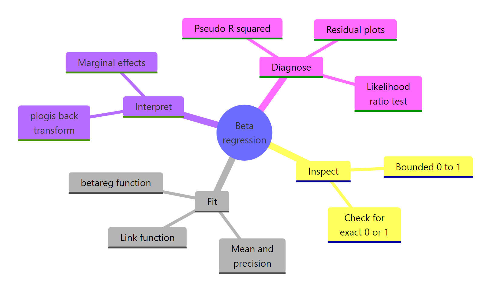
Beta regression workflow from data to diagnostics

Figure 2: The beta regression workflow from data to model to interpretation.

Concept	betareg syntax	When to use
Bounded response	`betareg(y ~ x, data = d)`	`y` is a continuous proportion in (0, 1)
Link function	`link = "logit"` (default), `"probit"`, `"cloglog"`	Logit for symmetric data, cloglog for skew
Variable precision	`y ~ x \	z`	Spread of `y` depends on covariate `z`
Back-transform coefficient	`plogis(coef)`	Convert logit-scale coefficient to response scale
Boundary 0 or 1	`(y * (n-1) + 0.5) / n`	A few exact 0s or 1s; large n
Model fit test	`lmtest::lrtest(m0, m1)`	Nested model comparison
Residual diagnostics	`plot(model, which = c(1, 4))`	Flag outliers and high-leverage points

References

Cribari-Neto, F., & Zeileis, A. (2010). Beta Regression in R. Journal of Statistical Software, 34(2). Link
Ferrari, S., & Cribari-Neto, F. (2004). Beta Regression for Modelling Rates and Proportions. Journal of Applied Statistics, 31(7), 799-815. Link
Smithson, M., & Verkuilen, J. (2006). A Better Lemon Squeezer? Maximum-likelihood regression with beta-distributed dependent variables. Psychological Methods, 11(1), 54-71. Link
CRAN betareg reference manual. Link
Grün, B., Kosmidis, I., & Zeileis, A. (2012). Extended Beta Regression in R: Shaken, Stirred, Mixed, and Partitioned. Journal of Statistical Software, 48(11). Link
Heiss, A. (2021). A guide to modeling proportions with Bayesian beta and zero-inflated beta regression models. Link
Mangiafico, S. R Companion Handbook: Beta Regression for Percent and Proportion Data. Link

Continue Learning

Logistic Regression in R, when the outcome is a binary 0/1, not a continuous proportion.
Poisson Regression in R, for modelling counts and rates with an offset.
Regression Diagnostics in R, deeper tools for residuals, leverage, and influence that extend to beta models.

Beta Regression in R: betareg Package for Proportions & Rates

When should you use beta regression instead of linear or logistic regression?

How does the beta distribution parameterize mean and precision?

How do you interpret betareg() coefficients on the logit scale?

How do you model variable precision (dispersion)?

How do you handle values exactly at 0 or 1?

How do you assess beta regression model fit?

Practice Exercises

Exercise 1: Variable-dispersion with AIC comparison

Exercise 2: Build a synthetic dataset with boundary values and recover the coefficient

Complete Example

Summary

References

Continue Learning

Related Tutorials