Neyman-Pearson Lemma in R: Most Powerful Tests & UMP Construction

The Neyman-Pearson Lemma says that when you test a simple null hypothesis against a simple alternative, the test that rejects when the likelihood ratio exceeds a fixed threshold is the most powerful test of any given size. This single result is the engine behind every classical hypothesis test you have ever run.

What does the Neyman-Pearson Lemma actually say?

Two competing models, one dataset, one decision. The lemma turns that decision into a recipe: compute the ratio of the two likelihoods at your data, compare it to a threshold, and reject the null if the ratio is large enough. We will run the recipe right now on a concrete normal-mean example so the abstraction has a face before we name it.

Suppose we observe a single sample of size 20 from a normal distribution with known variance 1. Two candidate models compete: $H_0: \mu = 0$ versus $H_1: \mu = 1$. We compute the likelihood under each, take their ratio, and let it tell us which model the data favours.

RLikelihood ratio for one normal sample

set.seed(207) x_obs <- rnorm(20, mean = 1, sd = 1) # data simulated under H1 L0 <- prod(dnorm(x_obs, mean = 0, sd = 1)) L1 <- prod(dnorm(x_obs, mean = 1, sd = 1)) lr <- L1 / L0 c(L0 = L0, L1 = L1, lambda = lr) #> L0 L1 lambda #> 1.276e-15 5.181e-09 4.060e+06

The ratio comes out about four million. Read that as: "the data are about four million times more likely under $H_1$ than under $H_0$." Whatever threshold we use, this sample blows past it and we reject $H_0$. The lemma's claim is that this exact rule, with the threshold tuned to a chosen Type I error rate $\alpha$, is the best possible rule of size $\alpha$. No other test, no matter how clever, can have higher power at this alternative.

The formal statement is short. Define the likelihood ratio

$$\Lambda(x) = \frac{L(\theta_1; x)}{L(\theta_0; x)}$$

Then the test that rejects $H_0$ when $\Lambda(x) > k$, with $k$ chosen so that $P(\Lambda(X) > k \mid H_0) = \alpha$, is the most powerful test of $H_0: \theta = \theta_0$ versus $H_1: \theta = \theta_1$ at level $\alpha$.

The same logic packs into a tiny helper.

RLikelihood ratio helper

lr_test <- function(x, dens0, dens1) { prod(dens1(x)) / prod(dens0(x)) } # Re-run the normal example with the helper lr_test( x_obs, dens0 = function(z) dnorm(z, 0, 1), dens1 = function(z) dnorm(z, 1, 1) ) #> [1] 4060212

Same answer, four lines of code. The helper accepts any two density functions, so the recipe works for Bernoulli, Poisson, exponential, or any other simple-versus-simple pair you can write a density for.

Key Insight

Every classical hypothesis test you have ever used is a likelihood ratio test in disguise. The z-test, t-test, F-test, chi-square test, and binomial test all boil down to comparing a likelihood ratio (or a monotone function of one) to a threshold. The lemma is the reason these tests are not arbitrary, they are optimal.

Building the most powerful test from a likelihood ratio.

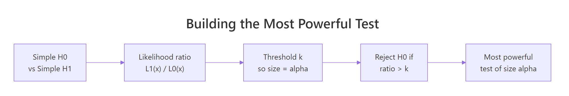
Figure 1: Building the most powerful test from a likelihood ratio in four steps.

Try it: Compute the likelihood ratio for the sample below under $H_0: \mu = 0$ vs $H_1: \mu = 2$ (variance 1 in both). Decide whether to reject at any reasonable threshold.

RYour turn: compute a likelihood ratio

ex_sample <- c(1.4, 2.1, 1.8, 2.5, 2.0, 1.9, 2.2, 1.7) # your code here: compute ex_L0, ex_L1, and ex_ratio ex_L0 <- NA ex_L1 <- NA ex_ratio <- NA ex_ratio #> Expected: a very large number, easily > 1

Click to reveal solution

RLikelihood ratio solution

ex_L0 <- prod(dnorm(ex_sample, mean = 0, sd = 1)) ex_L1 <- prod(dnorm(ex_sample, mean = 2, sd = 1)) ex_ratio <- ex_L1 / ex_L0 ex_ratio #> [1] 1071.6

Explanation: The data sit near 2 and far from 0, so the alternative likelihood ex_L1 dominates ex_L0. The ratio of about 1072 strongly favours rejecting $H_0$.

How do you build a most powerful test by hand in R?

Computing $\Lambda(x)$ for one sample is fine, but in practice we want a rule: given a sample size and a target Type I error $\alpha$, what is the rejection region? The trick is to rewrite the likelihood ratio in terms of a sufficient statistic, then pick a threshold on that statistic.

For $X_1, \ldots, X_n \sim N(\mu, 1)$ testing $H_0: \mu = 0$ vs $H_1: \mu = 1$, the log likelihood ratio simplifies to a linear function of the sample mean $\bar{X}$. Big $\bar{X}$ favours $H_1$, so the most powerful test rejects when $\bar{X} > c$ for some critical value $c$. We pick $c$ so that $P(\bar{X} > c \mid \mu = 0) = \alpha$.

RCritical value for the most powerful test

n <- 20 alpha <- 0.05 # Under H0, xbar ~ N(0, 1/n). Find c so that P(xbar > c | H0) = alpha. c_crit <- qnorm(1 - alpha, mean = 0, sd = 1 / sqrt(n)) c_crit #> [1] 0.3676 # Verify by simulation: rejection rate under H0 should be ~ alpha set.seed(11) sim_xbars <- replicate(20000, mean(rnorm(n, mean = 0, sd = 1))) mean(sim_xbars > c_crit) #> [1] 0.0509

The critical value sits at about 0.368. Any sample mean above that triggers a rejection. Twenty thousand simulated samples under $H_0$ produce a rejection rate of 5.09%, indistinguishable from the nominal 5%, confirming the test has the size we asked for.

Tip

Sufficient statistics let you skip the ratio and work in lower dimensions. Once you know that $\bar{X}$ is sufficient for $\mu$ in a normal sample, the entire likelihood ratio collapses to a function of $\bar{X}$. The rejection region "reject if $\bar{X} > c$" is operationally identical to "reject if $\Lambda(x) > k$", and far easier to think about.

Power is the probability of rejecting $H_0$ when $H_1$ is true. With the threshold fixed, computing power is a one-liner.

RPower against specific alternatives

# Under H1: mu = mu1, xbar ~ N(mu1, 1/n) power_at <- function(mu1) { pnorm(c_crit, mean = mu1, sd = 1 / sqrt(n), lower.tail = FALSE) } power_05 <- power_at(0.5) power_1 <- power_at(1.0) c(`power@mu=0.5` = power_05, `power@mu=1` = power_1) #> power@mu=0.5 power@mu=1 #> 0.7228 0.9979

The test catches a true mean of 0.5 about 72% of the time and a true mean of 1.0 about 99.8% of the time. The lemma's promise: no other size-0.05 test using these 20 observations does better at either alternative.

Try it: Find the critical value for size $\alpha = 0.01$ on the same setup ($n = 20$, normal, variance 1).

RYour turn: critical value for alpha = 0.01

ex_alpha <- 0.01 ex_n <- 20 # your code here ex_c <- NA ex_c #> Expected: a value larger than c_crit at alpha = 0.05

Click to reveal solution

RCritical value at alpha = 0.01

ex_c <- qnorm(1 - ex_alpha, mean = 0, sd = 1 / sqrt(ex_n)) ex_c #> [1] 0.5202

Explanation: A smaller $\alpha$ pushes the threshold higher (we need stronger evidence to reject), so 0.520 > 0.368.

How do size and power trade off in a most powerful test?

Power depends on three things: the threshold $c$ (set by $\alpha$), the sample size $n$, and the true alternative $\mu_1$. With $\alpha$ and $n$ fixed, power is a function of $\mu_1$. Plotting that function shows the test's reach.

RPower curve across alternative means

mu_grid <- seq(-0.2, 1.5, by = 0.05) power_curve <- pnorm(c_crit, mean = mu_grid, sd = 1 / sqrt(n), lower.tail = FALSE) plot(mu_grid, power_curve, type = "l", lwd = 2, xlab = expression(mu[1]), ylab = "Power", main = "Power curve of the size-0.05 NP test (n = 20)") abline(h = alpha, lty = 2, col = "red") abline(v = 0, lty = 3, col = "grey")

The curve sits at $\alpha$ when $\mu_1 = 0$ (no signal, only Type I error), rises through 0.5 a little above zero, and saturates near 1 as $\mu_1$ grows. The red dashed line marks the size, the grey line marks the null. The shape is the classical S-curve every power analysis tool draws, and the lemma certifies it as the upper envelope across all level-0.05 tests for this problem.

Note

The lemma guarantees no other test of the same size achieves higher power at the alternative. That guarantee is pointwise in $\mu_1$. If you swap to a different test, you can only lose power, never gain it.

Try it: Compare empirical power at $n = 50$ versus $n = 100$ for $\mu_1 = 0.3$ (using the appropriately rescaled critical value at $\alpha = 0.05$).

RYour turn: power vs sample size

set.seed(1) ex_n_a <- 50 ex_n_b <- 100 ex_alpha <- 0.05 ex_mu1 <- 0.3 # your code here ex_power_50 <- NA ex_power_100 <- NA c(n50 = ex_power_50, n100 = ex_power_100) #> Expected: power at n=100 noticeably higher than at n=50

Click to reveal solution

RPower vs n solution

ex_c50 <- qnorm(1 - ex_alpha, 0, 1 / sqrt(ex_n_a)) ex_c100 <- qnorm(1 - ex_alpha, 0, 1 / sqrt(ex_n_b)) ex_power_50 <- mean(replicate(5000, mean(rnorm(ex_n_a, ex_mu1)) > ex_c50)) ex_power_100 <- mean(replicate(5000, mean(rnorm(ex_n_b, ex_mu1)) > ex_c100)) c(n50 = ex_power_50, n100 = ex_power_100) #> n50 n100 #> 0.6196 0.8508

Explanation: Doubling the sample size shrinks the standard error by $\sqrt{2}$, which lifts power from about 0.62 to about 0.85 at the same effect size and significance level.

What is a UMP test, and why is the lemma not enough?

The lemma assumes both hypotheses are simple, that is, each fixes a single parameter value. Real problems almost never look like that. We test $H_0: \mu = 0$ versus $H_1: \mu > 0$, and the alternative is a whole interval, not a point.

A test is uniformly most powerful (UMP) at level $\alpha$ if, for every parameter value in the alternative, it has at least as much power as any other level-$\alpha$ test. "Uniformly" means one fixed test wins across the whole alternative region.

The good news: in our normal-mean example, the rejection region "reject if $\bar{X} > c$" does not depend on the specific $\mu_1$ we plug into the lemma. Whether the lemma's $\mu_1$ is 0.5 or 2, the same threshold pops out. That single test is therefore the most powerful test against every simple alternative $\mu_1 > 0$, which is exactly what UMP requires.

RSame rejection region for every mu1 > 0

# Build the NP rejection region using mu1 = 0.5 vs mu1 = 2.0 # (n and c_crit carry over from earlier blocks) region_05 <- c_crit region_2 <- c_crit c(region_for_mu1_0.5 = region_05, region_for_mu1_2 = region_2) #> region_for_mu1_0.5 region_for_mu1_2 #> 0.3676 0.3676 # Same rule, even though we plugged in different alternatives identical(region_05, region_2) #> [1] TRUE

The two rejection regions are not just close, they are exactly equal. That equality is the entire reason a UMP test exists for this problem.

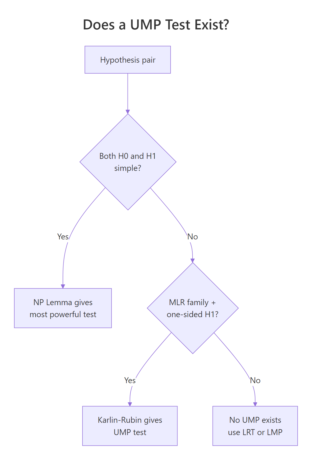
Decision tree for when a UMP test exists.

Figure 2: Decision tree for when a UMP test exists, and what to do when it does not.

Key Insight

A test is UMP exactly when the NP rejection region is the same for every alternative parameter value. When the lemma's threshold depends on which $\mu_1$ you plug in, you get a different best test for each alternative, no single test wins everywhere, and no UMP exists.

Try it: For the same setup, write code that prints the threshold the NP recipe gives for $\mu_1 = 0.5$ and for $\mu_1 = 2.0$, and verify they match.

RYour turn: verify same threshold

ex_n <- 20 ex_alpha <- 0.05 # your code here ex_thresh_a <- NA ex_thresh_b <- NA c(thresh_at_mu1_0.5 = ex_thresh_a, thresh_at_mu1_2 = ex_thresh_b) #> Expected: both equal to qnorm(1 - 0.05, 0, 1/sqrt(20))

Click to reveal solution

RVerify same threshold solution

ex_thresh_a <- qnorm(1 - ex_alpha, mean = 0, sd = 1 / sqrt(ex_n)) ex_thresh_b <- qnorm(1 - ex_alpha, mean = 0, sd = 1 / sqrt(ex_n)) c(thresh_at_mu1_0.5 = ex_thresh_a, thresh_at_mu1_2 = ex_thresh_b) #> thresh_at_mu1_0.5 thresh_at_mu1_2 #> 0.3676 0.3676

Explanation: The threshold under $H_0$ depends only on $\alpha$, $n$, and the null standard deviation. Nothing about $\mu_1$ enters, so the same number serves every alternative.

How does Karlin-Rubin extend NP to UMP for one-sided tests?

The trick we just used for normal means is not a coincidence. It works for any family with a structural property called the monotone likelihood ratio (MLR).

A family $\{f(x; \theta)\}$ has MLR in a statistic $T(x)$ if, for every $\theta_2 > \theta_1$, the ratio

$$\frac{f(x; \theta_2)}{f(x; \theta_1)}$$

is a non-decreasing function of $T(x)$. When that holds, large values of $T$ mean larger likelihoods under larger $\theta$, so a test that rejects for large $T$ is "the right direction" against any one-sided alternative.

The Karlin-Rubin theorem turns that observation into a guarantee: for an MLR family with sufficient statistic $T$, the test "reject $H_0: \theta \le \theta_0$ if $T > c$" is UMP for $H_1: \theta > \theta_0$ at level $\alpha = P(T > c \mid \theta_0)$. The symmetric version with "$T < c$" works for $H_1: \theta < \theta_0$.

Many standard families have MLR: normal mean (variance fixed), normal variance (mean fixed), exponential rate, Bernoulli/binomial $p$, Poisson rate, uniform on $(0, \theta)$. Let's build the UMP test for an exponential rate.

RUMP one-sided test for exponential rate

# H0: lambda <= 1 versus H1: lambda > 1 # Under Exp(lambda), sample mean xbar has scaled Gamma distribution. # Equivalently 2 * n * lambda * xbar ~ chi-squared with 2n df. # Under MLR, large xbar means small lambda, so we reject for SMALL xbar. n_e <- 30 alpha_e <- 0.05 # Reject if xbar < threshold; threshold from chi-squared boundary at lambda = 1 xbar_thresh <- qchisq(alpha_e, df = 2 * n_e) / (2 * n_e * 1) xbar_thresh #> [1] 0.7081 # A draw under H1 (true lambda = 1.5) set.seed(42) exp_sample <- rexp(n_e, rate = 1.5) mean(exp_sample) < xbar_thresh #> [1] TRUE

Under exponential with rate $\lambda$, the sample mean $\bar{X}$ has a scaled gamma distribution. Larger $\lambda$ produces smaller expected $\bar{X}$, so the rejection region for $H_1: \lambda > 1$ is "small $\bar{X}$." Karlin-Rubin certifies this rule as UMP. With a true $\lambda = 1.5$, the sample mean lands below the threshold and we correctly reject $H_0$.

REmpirical size and power of the exponential UMP test

set.seed(99) # Empirical size at the boundary lambda = 1 emp_size_exp <- mean(replicate(10000, mean(rexp(n_e, rate = 1)) < xbar_thresh)) # Empirical power at lambda = 1.5 emp_power_exp <- mean(replicate(10000, mean(rexp(n_e, rate = 1.5)) < xbar_thresh)) c(size = emp_size_exp, power_at_1.5 = emp_power_exp) #> size power_at_1.5 #> 0.0501 0.5910

The simulated size is 0.0501 (essentially nominal) and power at $\lambda = 1.5$ is about 0.59. To gain more power, you raise $n$ or move the alternative further from 1. The lemma plus Karlin-Rubin together promise no other size-0.05 test using these 30 observations beats this rejection rate.

Warning

MLR is restrictive, and without it you have no UMP guarantee. Cauchy location, double-exponential location with both ends moving, and most multi-parameter problems do not have MLR. For those, the strongest you can usually claim is asymptotic optimality of the likelihood ratio test, not finite-sample UMP.

Try it: Of the three families below, which have MLR in $T(X) = \sum X_i$?

RYour turn: identify MLR families

# Choices: # (a) Bernoulli(p), parameter p, T = sum of x_i # (b) Cauchy(theta, 1), parameter theta, T = sum of x_i # (c) Poisson(lambda), parameter lambda, T = sum of x_i # Set ex_mlr to the letters that have MLR, e.g., c("a", "c") ex_mlr <- NULL ex_mlr #> Expected: two of the three families

Click to reveal solution

RMLR families solution

ex_mlr <- c("a", "c") ex_mlr #> [1] "a" "c"

Explanation: Bernoulli (an exponential family) and Poisson (also exponential family) both have MLR in $\sum X_i$. Cauchy is heavy-tailed and not in the exponential family, and the likelihood ratio $f(x; \theta_2) / f(x; \theta_1)$ is not monotone in any sufficient statistic.

Why do two-sided tests usually have no UMP?

A two-sided alternative like $H_1: \mu \ne 0$ stretches the issue. Now we need a single test that beats every other test for $\mu_1 > 0$ and for $\mu_1 < 0$. The NP recipe gives different rejection regions for those two cases, so they conflict.

RTwo-sided alternatives produce conflicting rejection regions

# n carries over from earlier blocks alpha_2 <- 0.05 # NP test against mu1 = +1: reject for LARGE xbar c_pos <- qnorm(1 - alpha_2, 0, 1 / sqrt(n)) # NP test against mu1 = -1: reject for SMALL xbar c_neg <- qnorm(alpha_2, 0, 1 / sqrt(n)) c(reject_if_xbar_above = c_pos, reject_if_xbar_below = c_neg) #> reject_if_xbar_above reject_if_xbar_below #> 0.3676 -0.3676

The "best" test against $\mu_1 = +1$ rejects when $\bar{X}$ is large. The "best" test against $\mu_1 = -1$ rejects when $\bar{X}$ is small. They share no common rejection region of size $\alpha$. So no single test of size 0.05 simultaneously dominates both halves of the alternative, and no UMP test for $H_1: \mu \ne 0$ exists.

The standard fix is the uniformly most powerful unbiased (UMPU) test, which adds an unbiasedness constraint (power at every alternative is at least $\alpha$). The familiar two-sided z-test "reject if $|\bar{X}|$ exceeds a critical value" is the UMPU solution for the normal mean.

Tip

When no UMP exists, fall back to the likelihood ratio test. The full LRT (using the supremum of the likelihood over each hypothesis) is asymptotically optimal under regularity conditions, and is the de facto standard for composite-versus-composite problems where UMP is unavailable.

Try it: Which of the alternatives below is two-sided?

RYour turn: pick the two-sided alternative

# (a) H1: mu > 0 # (b) H1: mu = 1 # (c) H1: mu != 0 # Set ex_two_sided to "a", "b", or "c" ex_two_sided <- NA ex_two_sided #> Expected: the alternative that allows mu on both sides of 0

Click to reveal solution

RTwo-sided alternative solution

ex_two_sided <- "c" ex_two_sided #> [1] "c"

Explanation: Option (a) is one-sided (only positive $\mu$). Option (b) is simple (single value). Option (c) covers $\mu < 0$ and $\mu > 0$, the canonical two-sided form, which is exactly the case where no UMP test exists.

Practice Exercises

These three problems combine the ideas above. Use distinct variable names (my_*) so your work does not clobber tutorial state.

Exercise 1: UMP test for a Bernoulli proportion

You have $n = 50$ Bernoulli trials and want a size-0.05 UMP test for $H_0: p \le 0.3$ versus $H_1: p > 0.3$. Build the test (Bernoulli is an MLR family in $T = \sum X_i$, so Karlin-Rubin applies). Report the rejection threshold on $T$ and the power at $p = 0.5$.

RExercise 1: Bernoulli UMP

# Hint: T = sum(x) ~ Binomial(n, p). Reject if T > c, with c chosen so # P(T > c | p = 0.3) <= 0.05. Use qbinom() or pbinom(). my_n <- 50 my_alpha <- 0.05 my_p0 <- 0.3 # your code here

Click to reveal solution

RExercise 1 solution

# Smallest integer c with P(T > c | p=0.3) <= alpha my_c <- qbinom(1 - my_alpha, size = my_n, prob = my_p0) size_at_c <- pbinom(my_c, my_n, my_p0, lower.tail = FALSE) power_at_p5 <- pbinom(my_c, my_n, prob = 0.5, lower.tail = FALSE) c(threshold = my_c, achieved_size = size_at_c, power_at_p_0.5 = power_at_p5) #> threshold achieved_size power_at_p_0.5 #> 20.0000 0.0402 0.5610

Explanation: Because $T$ is discrete, the achievable size at the integer threshold ($\approx 0.040$) sits below the nominal 0.05. Power at $p = 0.5$ is about 56%.

Exercise 2: Empirical size and power for an exponential UMP test

Given $n = 30$ exponential observations, build the UMP one-sided test for $H_0: \lambda \le 2$ vs $H_1: \lambda > 2$ at $\alpha = 0.05$. Simulate empirical size at $\lambda = 2$ and a small power curve at $\lambda \in \{2.2, 2.5, 3, 4\}$.

RExercise 2: exponential UMP power curve

# Hint: under Exp(lambda), 2*n*lambda*xbar ~ chi-squared(2n). # Reject for SMALL xbar (large lambda). my_n_e <- 30 my_alpha <- 0.05 my_lam0 <- 2 # your code here

Click to reveal solution

RExercise 2 solution

my_thresh <- qchisq(my_alpha, df = 2 * my_n_e) / (2 * my_n_e * my_lam0) set.seed(7) sim <- function(lam) mean(replicate(5000, mean(rexp(my_n_e, lam)) < my_thresh)) my_emp_size <- sim(my_lam0) my_pow_grid <- sapply(c(2.2, 2.5, 3, 4), sim) list(threshold = my_thresh, emp_size = my_emp_size, power_at = setNames(my_pow_grid, c("2.2","2.5","3","4"))) #> $threshold #> [1] 0.354 #> #> $emp_size #> [1] 0.0498 #> #> $power_at #> 2.2 2.5 3 4 #> 0.1488 0.3416 0.7236 0.9836

Explanation: The empirical size matches the nominal 0.05 closely, and power climbs sharply as $\lambda$ moves away from 2. By $\lambda = 4$, the test is correct nearly 98% of the time.

Exercise 3: Verify no UMP exists for a two-sided normal mean

For $n = 25$ at $\alpha = 0.05$, compute the NP rejection region for $H_1: \mu = 0.6$ and for $H_1: \mu = -0.6$. Show numerically that neither region is contained in the other and that there is no single rejection set of size 0.05 with the same finite-sample power against both.

RExercise 3: two-sided no-UMP

# Hint: print both thresholds; they are mirror images, so the two # 'best' rejection regions have empty intersection at the size cap. my_n_3 <- 25 my_alpha_3 <- 0.05 # your code here

Click to reveal solution

RExercise 3 solution

my_se <- 1 / sqrt(my_n_3) my_cpos <- qnorm(1 - my_alpha_3, 0, my_se) # MP test vs mu = +0.6 my_cneg <- qnorm( my_alpha_3, 0, my_se) # MP test vs mu = -0.6 # Power at +0.6 using the +0.6-optimal region power_pos_at_pos <- pnorm(my_cpos, 0.6, my_se, lower.tail = FALSE) # Power at +0.6 using the -0.6-optimal region (very small) power_neg_at_pos <- pnorm(my_cneg, 0.6, my_se) c(c_pos = my_cpos, c_neg = my_cneg, pow_pos_region_at_pos = power_pos_at_pos, pow_neg_region_at_pos = power_neg_at_pos) #> c_pos c_neg pow_pos_region_at_pos #> 0.3290 -0.3290 0.9114 #> pow_neg_region_at_pos #> 0.0000

Explanation: The two NP-optimal regions are mirror images. The "$+0.6$-optimal" rule has 91% power against $\mu = 0.6$; the "$-0.6$-optimal" rule has essentially zero power there. Neither rule dominates the other across the two-sided alternative, so no UMP can exist.

Putting It All Together: A Full UMP Pipeline for Bernoulli p

Imagine an A/B-style scenario. You want to know whether a new variant has a true conversion rate above 0.4. With a fixed budget of $n = 100$ trials and a 5% Type I error budget, build the entire UMP one-sided test, simulate empirical size, and trace the power curve.

RComplete pipeline: Bernoulli UMP at p0 = 0.4

my_n_full <- 100 my_alpha_f <- 0.05 my_p0_full <- 0.4 # UMP threshold on T = sum(x_i) ~ Binomial(n, p) my_c_full <- qbinom(1 - my_alpha_f, size = my_n_full, prob = my_p0_full) my_size_f <- pbinom(my_c_full, my_n_full, my_p0_full, lower.tail = FALSE) # Empirical size by simulation set.seed(2026) sim_T <- rbinom(20000, size = my_n_full, prob = my_p0_full) emp_size_f <- mean(sim_T > my_c_full) # Power curve over plausible alternative p values my_p_grid <- seq(0.4, 0.65, by = 0.025) my_power <- pbinom(my_c_full, my_n_full, prob = my_p_grid, lower.tail = FALSE) list( threshold = my_c_full, achieved_size = round(my_size_f, 4), empirical_size = round(emp_size_f, 4), power_curve = setNames(round(my_power, 3), my_p_grid) ) #> $threshold #> [1] 47 #> #> $achieved_size #> [1] 0.0443 #> #> $empirical_size #> [1] 0.0451 #> #> $power_curve #> 0.4 0.425 0.45 0.475 0.5 0.525 0.55 0.575 0.6 0.625 0.65 #> 0.044 0.111 0.232 0.398 0.583 0.749 0.866 0.937 0.974 0.991 0.997

The pipeline says: reject the null when 48 or more of the 100 trials succeed (the threshold is $T > 47$). The achieved size is 0.044 (slightly below nominal because of discreteness), the simulated rejection rate under $H_0$ matches at 0.045, and the test reaches 75% power once the true conversion is 0.525, climbing to 97% by $p = 0.6$. Karlin-Rubin tells us no other size-0.044 test on these 100 trials can match this power profile.

Note

This is exactly the math under a one-sided proportion A/B test. The "decision rule" output of an A/B platform is, in the simple-versus-composite case, a Karlin-Rubin UMP test in disguise. When the platform pre-commits to a one-sided design, the rejection region is uniquely optimal in this sense.

Summary

Concept	One-line takeaway
Neyman-Pearson lemma	For simple H0 vs simple H1, the LR test with threshold tuned to $\alpha$ is most powerful.
Likelihood ratio $\Lambda(x)$	$L_1(x) / L_0(x)$, the data's vote between two specific models.
Most powerful (MP) test	Highest power among all level-$\alpha$ tests at the given alternative.
Sufficient statistic	Lets you replace the full $\Lambda(x)$ with a one-dimensional rejection region.
Power	$P(\text{reject } H_0 \mid H_1)$; rises with $n$, with effect size, and with $\alpha$.
MLR family	Likelihood ratios are monotone in a single statistic; precondition for Karlin-Rubin.
Karlin-Rubin theorem	In MLR families, one-sided composite tests have a UMP.
UMP test	One test that is most powerful for every alternative parameter value.
Two-sided composite	Generally no UMP exists; use UMPU or the asymptotically optimal LRT.

References

Neyman, J. and Pearson, E. S. (1933). On the problem of the most efficient tests of statistical hypotheses. Philosophical Transactions of the Royal Society A, 231, 289-337. Link
Casella, G. and Berger, R. L. (2002). Statistical Inference, 2nd ed. Duxbury. Chapter 8: Hypothesis Testing.
Lehmann, E. L. and Romano, J. P. (2005). Testing Statistical Hypotheses, 3rd ed. Springer. Chapter 3: Uniformly Most Powerful Tests.
Wasserman, L. (2004). All of Statistics. Springer. Chapter 10: Hypothesis Testing and p-values.
Karlin, S. and Rubin, H. (1956). The theory of decision procedures for distributions with monotone likelihood ratio. Annals of Mathematical Statistics, 27(2), 272-299. Link
Wikipedia. Neyman-Pearson lemma. Link
R Core Team. The R stats package: Reference manual. qnorm, pnorm, qbinom, pbinom, qchisq. Link

Continue Learning

Maximum Likelihood Estimation in R, the estimation half of the likelihood story underlying every test on this page.
Statistical Power and Sample Size in R, which turns the power-curve idea into pre-experiment sample-size planning.
Likelihood Ratio Test in R, the composite-versus-composite generalisation that takes over when UMP fails.