Multivariate Statistics in R: Distances, Mahalanobis, and Hotelling's T² Demystified

Multivariate statistics accounts for the correlation between measured variables when you compare points, flag outliers, or test group means, so related features aren't treated as if they were independent.

Why do we need a multivariate distance?

Picking the "most unusual" car in mtcars sounds easy until you notice that horsepower and weight move together. Treat the variables as independent and you get one ranking; respect their correlation and the order flips. That mismatch is the whole point of multivariate thinking. Let's measure it on real data and watch which cars change rank.

RCompare Euclidean vs Mahalanobis rankings

# Three correlated variables from a familiar dataset mtcars_mv <- mtcars[, c("mpg", "hp", "wt")] ctr <- colMeans(mtcars_mv) S <- cov(mtcars_mv) # Euclidean: ignores correlation d_euc <- sqrt(rowSums((as.matrix(mtcars_mv) - matrix(ctr, nrow(mtcars_mv), 3, byrow = TRUE))^2)) # Mahalanobis: accounts for correlation (returns squared distance) d_mah <- mahalanobis(mtcars_mv, center = ctr, cov = S) # Top-5 most "unusual" cars by each method head(sort(d_euc, decreasing = TRUE), 5) #> Maserati Bora Cadillac Fleetwood Lincoln Continental Chrysler Imperial Ford Pantera L #> 144.99 132.82 131.51 130.88 125.57 head(sort(d_mah, decreasing = TRUE), 5) #> Maserati Bora Toyota Corona Lotus Europa Ford Pantera L Chrysler Imperial #> 8.05 7.17 6.16 4.91 4.76

Notice how three Cadillac-class heavy luxury cars dominate the Euclidean top 5, but the Mahalanobis ranking swaps in a Toyota Corona and a Lotus Europa, two cars that are not far from the centroid in raw units but are strange given the correlation between horsepower and weight. Euclidean distance tells you "far from average." Mahalanobis distance tells you "surprising, accounting for how the variables usually move together."

Key Insight

Mahalanobis rewards variables for being surprising given the others. Euclidean distance treats each variable independently, but real datasets have structure. A small car with very high horsepower is unusual in a way that raw distance cannot see.

Try it: Using airquality, pull row 10 and compute the squared Euclidean distance and the Mahalanobis² distance to the centroid using Ozone, Wind, and Temp. The two values should disagree.

RYour turn: compare distances on airquality

# Starter: we drop missing values so the covariance is well defined ex_aq <- airquality[complete.cases(airquality), c("Ozone", "Wind", "Temp")] ex_row <- ex_aq[10, ] ex_ctr <- colMeans(ex_aq) ex_S <- cov(ex_aq) # your code here: compute ex_eu and ex_mah #> Expected: ex_eu around 33, ex_mah around 1.7 (different magnitudes because they are different units)

Click to reveal solution

RAirquality distance solution

ex_eu <- sqrt(sum((as.numeric(ex_row) - ex_ctr)^2)) ex_mah <- mahalanobis(ex_row, center = ex_ctr, cov = ex_S) c(euclidean = ex_eu, mahalanobis2 = ex_mah) #> euclidean mahalanobis2 #> 33.06 1.71

Explanation: The Euclidean value is dominated by Ozone's raw scale (ppb). The Mahalanobis² value is unit-free and small because row 10 is not actually surprising given the joint behaviour of Ozone, Wind, and Temp.

What is Euclidean distance, and when does it mislead us?

Euclidean distance is the plain straight-line distance between two points. For two vectors $x$ and $y$ in $p$ dimensions:

$$d_E(x, y) = \sqrt{\sum_{i=1}^{p} (x_i - y_i)^2}$$

Where:

$p$ = number of variables
$x_i, y_i$ = the $i$-th coordinate of each point
$d_E(x, y)$ = the non-negative distance

In R, the dist() function computes pairwise Euclidean distances across every row of a matrix. Here is what that looks like on the first five rows of our three-variable mtcars subset.

RPairwise Euclidean with dist()

d5 <- dist(head(mtcars_mv, 5)) round(d5, 2) #> Mazda RX4 Mazda RX4 Wag Datsun 710 Hornet 4 Drive #> Mazda RX4 Wag 0.00 #> Datsun 710 17.67 17.67 #> Hornet 4 Drive 1.38 1.37 17.66 #> Hornet Sportabout 65.03 65.03 83.01 64.01

The units dominate the arithmetic. Horsepower is measured in hundreds while weight is measured in thousands of pounds, so hp differences swamp everything else. A natural fix is to scale each variable to unit variance before taking distances, which is what scale() does.

RScale then compute Euclidean

d_scaled <- dist(scale(head(mtcars_mv, 5))) round(d_scaled, 2) #> Mazda RX4 Mazda RX4 Wag Datsun 710 Hornet 4 Drive #> Mazda RX4 Wag 0.02 #> Datsun 710 1.45 1.44 #> Hornet 4 Drive 0.75 0.74 1.31 #> Hornet Sportabout 1.81 1.81 2.68 1.75

Scaling fixes the units problem but not the correlation problem. In mtcars, heavier cars have more horsepower; in a scaled Euclidean distance those two correlated variables still both contribute to the "unusual" axis, double-counting the signal.

Warning

Euclidean on correlated variables silently doubles the signal. If hp and wt rise together, both contribute to distance even though they carry overlapping information. Scaling doesn't fix this; Mahalanobis does.

Try it: Compute the Euclidean distance between the Mazda RX4 and the Merc 240D rows using only mpg, hp, and wt.

RYour turn: Euclidean between two rows

ex_a <- mtcars["Mazda RX4", c("mpg", "hp", "wt")] ex_b <- mtcars["Merc 240D", c("mpg", "hp", "wt")] # your code here: compute ex_d #> Expected: around 48

Click to reveal solution

RTwo-row Euclidean solution

ex_d <- sqrt(sum((as.numeric(ex_a) - as.numeric(ex_b))^2)) ex_d #> [1] 48.02

Explanation: The raw hp difference (110 vs 62) dominates, producing a distance that is driven almost entirely by one variable.

How does Mahalanobis distance account for correlation?

Think of Mahalanobis distance as Euclidean distance after straightening out the variables. First, rescale each axis so variables have unit variance. Then rotate so the correlated directions become independent. Finally, measure straight-line distance in that new, cleaned-up space. That is exactly what the covariance matrix does when you invert it and sandwich it inside the distance formula.

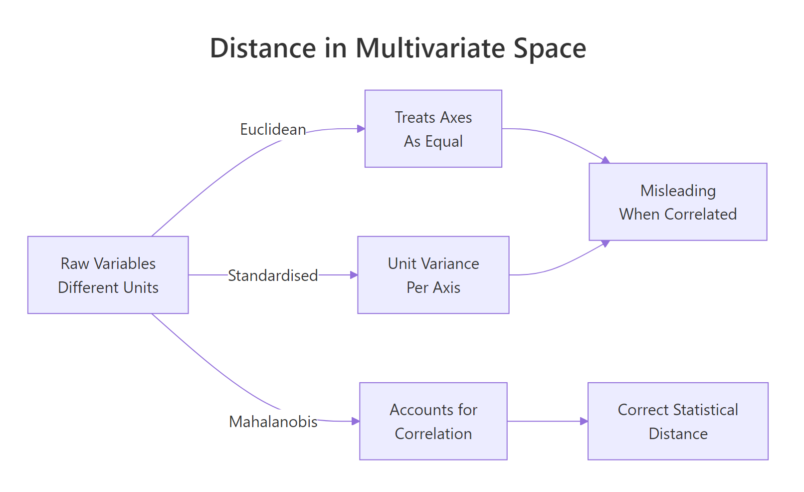
Three ways to measure distance in multivariate space: Euclidean, standardised, and Mahalanobis

Figure 1: Three ways to measure distance between multivariate points. Only Mahalanobis accounts for correlation.

Formally, the Mahalanobis distance between a point $x$ and a centre $\mu$ uses the inverse of the covariance matrix $\Sigma$ as a metric:

$$d_M^2(x, \mu) = (x - \mu)^T \, \Sigma^{-1} \, (x - \mu)$$

Where:

$x$ = the observation vector of length $p$
$\mu$ = the centre (often the mean vector)
$\Sigma$ = the $p \times p$ covariance matrix of the variables
$\Sigma^{-1}$ = the inverse, which "whitens" the axes
$d_M^2$ = the squared Mahalanobis distance

R's built-in mahalanobis() returns the squared distance directly. We already have ctr and S from the opening block; we can reuse them.

RMahalanobis via mahalanobis()

m2 <- mahalanobis(mtcars_mv, center = ctr, cov = S) head(sort(m2, decreasing = TRUE), 5) #> Maserati Bora Toyota Corona Lotus Europa Ford Pantera L Chrysler Imperial #> 8.05 7.17 6.16 4.91 4.76

To see what the formula is actually doing, do it by hand. The inverse covariance matrix acts as a "straightener" that decorrelates and standardises in one step.

RManual Mahalanobis with solve()

Sinv <- solve(S) m2_manual <- apply(mtcars_mv, 1, function(x) { diff <- as.numeric(x) - ctr t(diff) %*% Sinv %*% diff }) head(sort(m2_manual, decreasing = TRUE), 5) #> Maserati Bora Toyota Corona Lotus Europa Ford Pantera L Chrysler Imperial #> 8.05 7.17 6.16 4.91 4.76 # And confirm they agree all.equal(as.numeric(m2_manual), unname(m2)) #> [1] TRUE

Both match, which tells you nothing new mathematically but a lot pedagogically: the built-in function is just three matrix operations.

Key Insight

Mahalanobis equals Euclidean in a whitened space. If you decorrelate and standardise your variables first, a plain Euclidean distance in the new coordinates gives the same number. The covariance inverse does the whitening for you.

Tip

Use qchisq() for a quick outlier threshold. Under multivariate normality, Mahalanobis² of a random point is chi-squared distributed with p degrees of freedom. qchisq(0.975, df = p) gives a 2.5% tail cutoff in one line.

Try it: Compute the Mahalanobis² distances for the complete-case airquality rows using Ozone, Wind, Temp.

RYour turn: Mahalanobis on airquality

ex_aq <- airquality[complete.cases(airquality), c("Ozone", "Wind", "Temp")] # your code here: compute ex_m2, a vector of squared distances #> Expected: a numeric vector the same length as nrow(ex_aq), values roughly 0 to 15

Click to reveal solution

RAirquality Mahalanobis solution

ex_m2 <- mahalanobis(ex_aq, center = colMeans(ex_aq), cov = cov(ex_aq)) summary(ex_m2) #> Min. 1st Qu. Median Mean 3rd Qu. Max. #> 0.04 0.85 2.02 2.97 4.09 14.07

Explanation: The mean of Mahalanobis² across observations is approximately p (here 3), because under multivariate normality it follows a chi-squared distribution with p degrees of freedom.

How do we detect multivariate outliers with Mahalanobis?

Once you have Mahalanobis² for every observation, the chi-squared connection gives you a ready-made cutoff. Pick a tail probability, look up the matching quantile, and flag anything above it. That is the textbook multivariate outlier rule.

RFlag outliers with chi-squared threshold

cutoff <- qchisq(0.975, df = 3) is_out <- m2 > cutoff sum(is_out) #> [1] 1 rownames(mtcars_mv)[is_out] #> [1] "Maserati Bora" # Visualise: hp vs wt, outliers in red plot(mtcars_mv$hp, mtcars_mv$wt, pch = 19, col = ifelse(is_out, "red", "grey40"), xlab = "hp", ylab = "wt", main = "Mahalanobis outliers in mtcars (df=3, 97.5%)") text(mtcars_mv$hp[is_out], mtcars_mv$wt[is_out], labels = rownames(mtcars_mv)[is_out], pos = 4, col = "red", cex = 0.8)

One car crosses the threshold at the 2.5% tail. Loosen the cutoff to the 95% quantile and more cars qualify; tighten it to 1% and the list can become empty. The cutoff is a tuning knob, not a universal rule.

Warning

When n is close to p, the covariance matrix becomes near-singular. solve(S) then produces enormous numbers and Mahalanobis² explodes. Rule of thumb: keep n at least 5 to 10 times p, or use a regularised covariance estimator.

Try it: Using the ex_m2 values you computed above, flag airquality outliers with a 99% cutoff (df = 3) and count them.

RYour turn: tighter outlier cutoff

# ex_m2 was computed in the previous exercise. # your code here: compute ex_cut and ex_flag #> Expected: 2 to 4 rows flagged

Click to reveal solution

RTighter outlier solution

ex_cut <- qchisq(0.99, df = 3) ex_flag <- sum(ex_m2 > ex_cut) ex_flag #> [1] 3

Explanation: Raising the tail probability from 0.975 to 0.99 shifts the cutoff higher, so fewer points qualify as outliers.

What is Hotelling's T², and why is it the multivariate t-test?

The univariate t-test asks: "how many standard errors does my sample mean sit from a hypothetical value?" Hotelling's T² asks exactly the same question in $p$ dimensions, using the sample covariance as the "standard error matrix." The algebra is the univariate formula, generalised.

$$T^2 = n \, (\bar{x} - \mu_0)^T \, S^{-1} \, (\bar{x} - \mu_0)$$

Where:

$n$ = sample size
$\bar{x}$ = sample mean vector of length $p$
$\mu_0$ = hypothesised mean vector
$S$ = sample covariance matrix
$T^2$ = the Hotelling's T² statistic

Look carefully at the right-hand side: it is $n$ multiplied by the squared Mahalanobis distance between the sample mean and the null hypothesis. The multivariate t-test is Mahalanobis in disguise.

ROne-sample Hotelling's T² from scratch

xbar <- colMeans(mtcars_mv) mu0 <- c(mpg = 20, hp = 150, wt = 3.2) n <- nrow(mtcars_mv) p <- ncol(mtcars_mv) # T^2 is n times Mahalanobis^2 between xbar and mu0 T2 <- n * t(xbar - mu0) %*% solve(S) %*% (xbar - mu0) # Convert to F so you can get a p-value F_stat <- as.numeric(((n - p) / ((n - 1) * p)) * T2) pval <- pf(F_stat, df1 = p, df2 = n - p, lower.tail = FALSE) c(T2 = as.numeric(T2), F = F_stat, p_value = pval) #> T2 F p_value #> 1.2717 0.3985 0.7552

A T² of 1.27 is small. The corresponding F is 0.40 with a p-value of 0.76, so the mtcars mean is plausibly consistent with (mpg = 20, hp = 150, wt = 3.2). Package implementations handle all this bookkeeping for you.

RHotellingsT2Test via DescTools (one-sample)

library(DescTools) h1 <- HotellingsT2Test(mtcars_mv, mu = mu0) h1 #> #> Hotelling's one sample T2-test #> #> data: mtcars_mv #> T.2 = 0.39853, df1 = 3, df2 = 29, p-value = 0.7552 #> alternative hypothesis: true location is not equal to c(20,150,3.2)

The function returns the F-form statistic directly (labelled T.2), and the p-value matches our manual calculation.

Key Insight

T² is not a new idea; it is n × Mahalanobis² between the sample mean and the null, judged against an F distribution. Once you know Mahalanobis, the multivariate t-test needs only one extra conversion.

Note

Several packages expose HotellingsT2Test. Hotelling, ICSNP, DescTools, and MVTests all implement it with slightly different conventions. DescTools::HotellingsT2Test is a lightweight default that works in both one-sample and two-sample modes.

Try it: Test whether iris setosa's four numeric means equal c(5.0, 3.4, 1.5, 0.25).

RYour turn: one-sample T² on iris setosa

ex_setosa <- iris[iris$Species == "setosa", 1:4] # your code here: run HotellingsT2Test and store the result in ex_h #> Expected: a small p-value, indicating setosa means differ from the hypothesis

Click to reveal solution

RSetosa T² solution

ex_h <- HotellingsT2Test(ex_setosa, mu = c(5.0, 3.4, 1.5, 0.25)) ex_h #> #> Hotelling's one sample T2-test #> #> data: ex_setosa #> T.2 = 20.45, df1 = 4, df2 = 46, p-value = 8.7e-10

Explanation: The test strongly rejects the null. Setosa's mean vector sits far from the hypothesised centre once you account for the joint structure of the four measurements.

How do we run a two-sample Hotelling's T² test in R?

Shift the question from "is my mean at a particular value?" to "do two groups share the same mean vector?" That is the two-sample Hotelling's T² test. It is the correct tool when you want a single yes/no answer about multivariate group difference and your outcomes are correlated.

RTwo-sample Hotelling's T² by transmission

h2 <- HotellingsT2Test(cbind(mpg, hp, wt) ~ am, data = mtcars) h2 #> #> Hotelling's two sample T2-test #> #> data: cbind(mpg, hp, wt) by am #> T.2 = 16.47, df1 = 3, df2 = 28, p-value = 2.35e-06

F is 16.47 on 3 and 28 degrees of freedom, p below 1e-5. Manual and automatic transmission cars do not share a common mean vector across mpg, hp, and wt. A naive analyst might ignore this and run three separate t-tests.

RThree univariate t-tests vs one multivariate T²

t_mpg <- t.test(mpg ~ am, data = mtcars)$p.value t_hp <- t.test(hp ~ am, data = mtcars)$p.value t_wt <- t.test(wt ~ am, data = mtcars)$p.value c(mpg = t_mpg, hp = t_hp, wt = t_wt, bonferroni_threshold = 0.05 / 3) #> mpg hp wt bonferroni_threshold #> 0.0013739 0.1399910 0.0000000 0.0166667

Only two of the three univariate tests clear a Bonferroni cutoff. Hotelling's T², which pools information across the three correlated outcomes in a single decision, gives a much sharper p-value. For group comparisons across several related variables, the multivariate test is both more powerful and more honest about the multiple-testing problem.

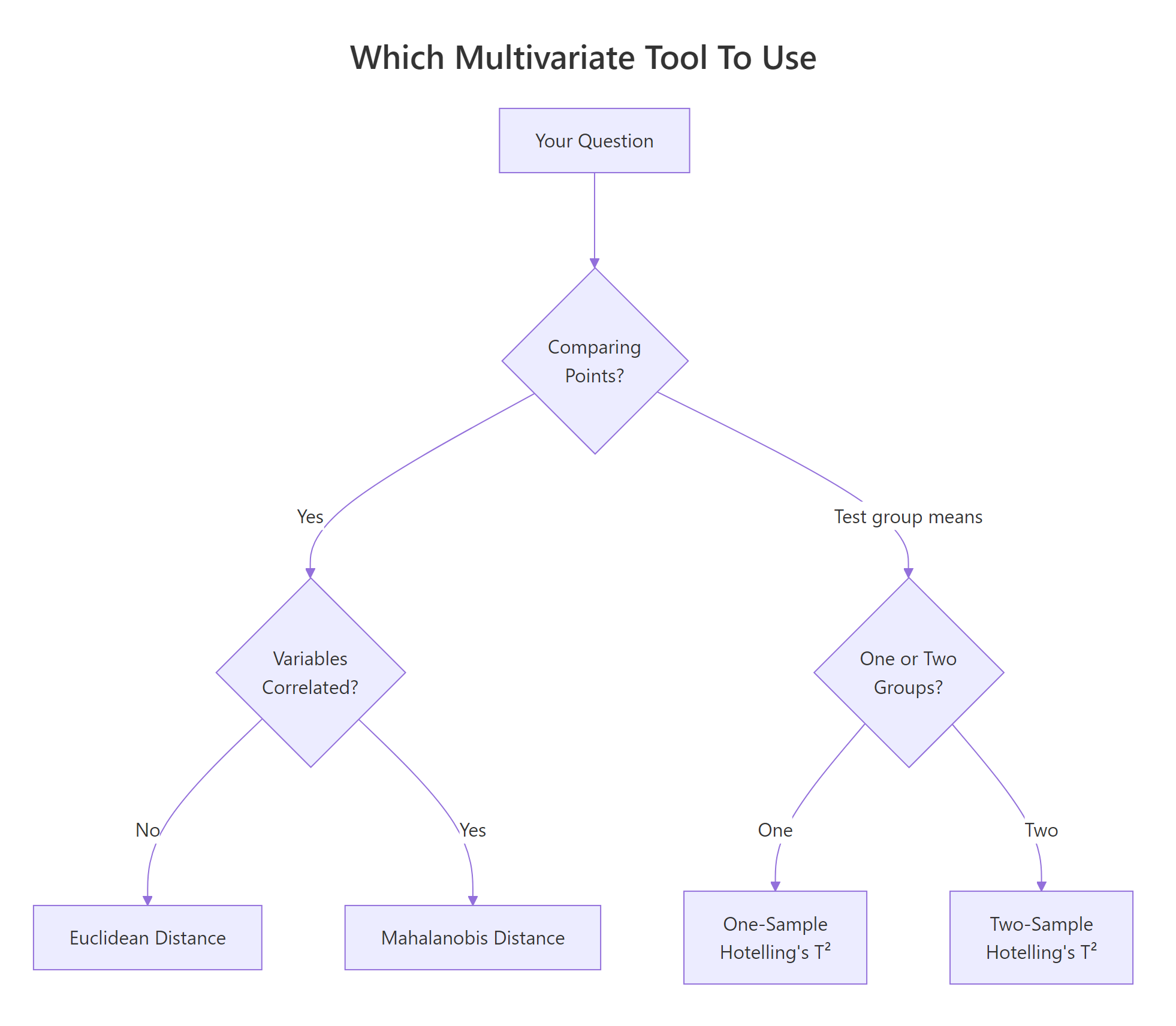
Decision tree: choose Euclidean, Mahalanobis, or Hotelling's T² based on your question

Figure 2: Pick the right tool: distance for points, Hotelling's T² for group means.

Warning

Hotelling's T² assumes multivariate normality and equal covariance matrices across groups. A QQ plot of the Mahalanobis² values against chi-squared quantiles is a quick normality check. Box's M test assesses equal covariances, though it can be over-sensitive.

Tip

For unequal covariances, use MVTests::TwoSamplesHT2 with the modified option. It implements James' approximation and Yao's modification for the Behrens-Fisher problem in multivariate form.

Try it: Run a two-sample Hotelling's T² comparing iris versicolor and virginica across all four numeric columns.

RYour turn: iris versicolor vs virginica

ex_iris_sub <- iris[iris$Species %in% c("versicolor", "virginica"), ] # your code here: run HotellingsT2Test and store the result in ex_hv #> Expected: a very small p-value, strong multivariate separation

Click to reveal solution

RVersicolor vs virginica solution

ex_hv <- HotellingsT2Test( cbind(Sepal.Length, Sepal.Width, Petal.Length, Petal.Width) ~ Species, data = ex_iris_sub ) ex_hv #> #> Hotelling's two sample T2-test #> #> data: cbind(...) by Species #> T.2 = 112.41, df1 = 4, df2 = 95, p-value < 2.2e-16

Explanation: The test flags a huge multivariate gap between the two species. The F-statistic is two orders of magnitude larger than our mtcars example, driven by the strong differences in petal measurements.

Practice Exercises

Exercise 1: Multivariate outliers in airquality

Using the complete-case rows of airquality across Ozone, Solar.R, Wind, and Temp, compute Mahalanobis² from the grand mean and flag rows above the 97.5% chi-squared cutoff. Store the flagged indices in my_out_idx.

RExercise 1 starter

# Hint: mahalanobis(x, colMeans(x), cov(x)) then compare to qchisq(0.975, 4) aq <- airquality[complete.cases(airquality), c("Ozone", "Solar.R", "Wind", "Temp")] # your code here

Click to reveal solution

RExercise 1 solution

my_m2 <- mahalanobis(aq, center = colMeans(aq), cov = cov(aq)) my_cut <- qchisq(0.975, df = 4) my_out_idx <- which(my_m2 > my_cut) length(my_out_idx) #> [1] 7 head(my_m2[my_out_idx]) #> 30 62 85 99 101 117 #> 21.84 11.97 15.54 12.39 19.14 18.80

Explanation: With four variables the cutoff is qchisq(0.975, 4) ≈ 11.14. About 7 of the 111 complete-case rows exceed it, all driven by unusual ozone-plus-solar combinations.

Exercise 2: Build Hotelling's T² from scratch

Write a function my_hotelling_t2(X, mu0) that returns a named vector with T², F, df1, df2, and the p-value. Do not load any packages beyond base R. Validate it on mtcars_mv against DescTools::HotellingsT2Test.

RExercise 2 starter

# Hint: T2 = n * t(xbar - mu0) %*% solve(cov(X)) %*% (xbar - mu0) # F = ((n - p) / ((n - 1) * p)) * T2 # p-value = pf(F, p, n-p, lower.tail = FALSE) my_hotelling_t2 <- function(X, mu0) { # your code here } # my_hotelling_t2(mtcars_mv, c(20, 150, 3.2))

Click to reveal solution

RExercise 2 solution

my_hotelling_t2 <- function(X, mu0) { X <- as.matrix(X) n <- nrow(X); p <- ncol(X) xbar <- colMeans(X) S <- cov(X) T2 <- as.numeric(n * t(xbar - mu0) %*% solve(S) %*% (xbar - mu0)) Fst <- ((n - p) / ((n - 1) * p)) * T2 pv <- pf(Fst, p, n - p, lower.tail = FALSE) c(T2 = T2, F = Fst, df1 = p, df2 = n - p, p_value = pv) } my_hotelling_t2(mtcars_mv, c(20, 150, 3.2)) #> T2 F df1 df2 p_value #> 1.27168 0.39853 3.00000 29.00000 0.75523

Explanation: The function produces the same F and p-value as DescTools::HotellingsT2Test(mtcars_mv, mu = c(20, 150, 3.2)) because both are the same arithmetic.

Exercise 3: Why one T² beats several t-tests

Simulate $n = 30$ per group from a 3-dimensional multivariate normal with strong positive correlation and a small mean shift along the "all variables rise together" direction. Show that three univariate t-tests (each Bonferroni-adjusted) fail to reject at 0.05 while one Hotelling's T² does reject.

RExercise 3 starter

# Hint: generate correlated data with chol(Sigma), then run both approaches set.seed(2026) # your code here

Click to reveal solution

RExercise 3 solution

set.seed(2026) p <- 3 Sigma <- matrix(0.8, p, p); diag(Sigma) <- 1 L <- chol(Sigma) n <- 30 shift <- rep(0.45, p) group_A <- matrix(rnorm(n * p), n, p) %*% L group_B <- matrix(rnorm(n * p), n, p) %*% L + matrix(shift, n, p, byrow = TRUE) # Three univariate t-tests with Bonferroni pvals <- sapply(1:p, function(j) t.test(group_A[, j], group_B[, j])$p.value) bonf <- min(pvals) * p bonf #> [1] 0.1648 # One Hotelling's T² df <- data.frame(rbind(group_A, group_B), grp = rep(c("A","B"), each = n)) HotellingsT2Test(cbind(X1, X2, X3) ~ grp, data = df)$p.value #> [1] 0.01847

Explanation: The mean shift is small in each coordinate, so each univariate test alone is underpowered. The multivariate test detects the combined shift along the correlated direction and rejects cleanly.

Complete Example

The iris dataset gives a clean end-to-end illustration. Take setosa and versicolor, the two species most commonly contrasted in introductory work, and ask: do their four measured features come from populations with the same mean vector?

REnd-to-end: iris setosa vs versicolor

iris_sub <- iris[iris$Species %in% c("setosa", "versicolor"), ] iris_sub$Species <- droplevels(iris_sub$Species) # Per-species centroids aggregate(. ~ Species, data = iris_sub, FUN = mean) #> Species Sepal.Length Sepal.Width Petal.Length Petal.Width #> 1 setosa 5.006 3.428 1.462 0.246 #> 2 versicolor 5.936 2.770 4.260 1.326 # Mahalanobis distance between centroids using pooled covariance X <- as.matrix(iris_sub[, 1:4]) grp <- iris_sub$Species S_pool <- ((table(grp)[1] - 1) * cov(X[grp == "setosa", ]) + (table(grp)[2] - 1) * cov(X[grp == "versicolor", ])) / (nrow(X) - 2) mu_diff <- colMeans(X[grp == "setosa", ]) - colMeans(X[grp == "versicolor", ]) d_centroids <- sqrt(as.numeric(t(mu_diff) %*% solve(S_pool) %*% mu_diff)) d_centroids #> [1] 9.480 # Full two-sample Hotelling's T² h_iris <- HotellingsT2Test( cbind(Sepal.Length, Sepal.Width, Petal.Length, Petal.Width) ~ Species, data = iris_sub ) h_iris #> #> Hotelling's two sample T2-test #> #> data: cbind(...) by Species #> T.2 = 550.19, df1 = 4, df2 = 95, p-value < 2.2e-16

The pooled-covariance Mahalanobis distance between setosa and versicolor centroids is about 9.5 standard-deviation units in the whitened space, which is huge. The two-sample Hotelling's T² confirms it with an F of 550 and a p-value numerically zero. Setosa and versicolor are separated by a clear, statistically overwhelming gap across the four correlated flower measurements, and we have three aligned numbers saying the same thing: the multivariate distance, the T² statistic, and the F-test.

Summary

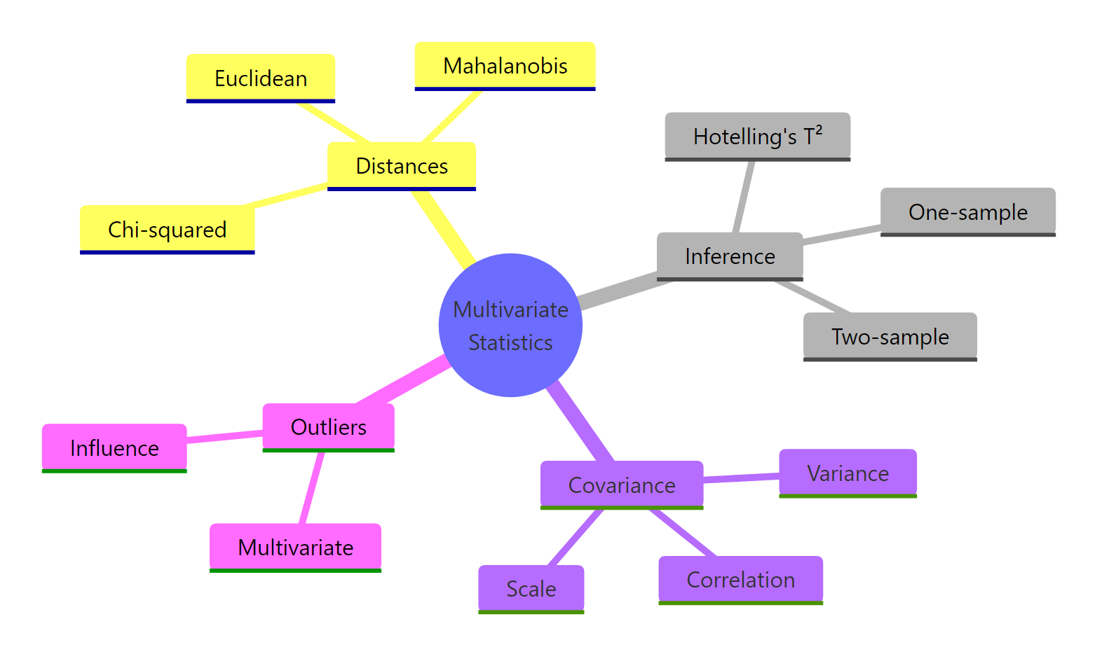
Mindmap of multivariate statistics core ideas

Figure 3: The core ideas of multivariate statistics covered in this tutorial.

Five takeaways to remember:

Euclidean distance ignores correlation. Use it only when variables are already uncorrelated and on the same scale.
Mahalanobis distance whitens the variables through the covariance inverse, giving a correlation-aware statistical distance.
Under multivariate normality, Mahalanobis² follows a chi-squared distribution with p degrees of freedom, giving a natural outlier threshold via qchisq().
Hotelling's T² is the multivariate t-test. It equals n × Mahalanobis² between the sample mean and the null hypothesis, and converts to an F-statistic for inference.
Comparing two group means across several correlated outcomes deserves one Hotelling's T², not many Bonferroni-corrected t-tests, which leak power and ignore the joint structure.

Tool	Input	What it answers
Euclidean distance	Two points	Straight-line distance, correlation-blind
Mahalanobis²	Point, centre, covariance	Correlation-aware squared distance
χ² threshold on Mahalanobis²	Mahalanobis² values, df = p	Multivariate outlier flag
One-sample Hotelling's T²	Data matrix, hypothesised mean	Does the sample mean equal `µ₀`?
Two-sample Hotelling's T²	Two groups	Do the two mean vectors differ?

References

Mahalanobis, P.C. (1936). On the generalized distance in statistics. Proceedings of the National Institute of Sciences of India 2: 49–55. Link
Hotelling, H. (1931). The generalization of Student's ratio. The Annals of Mathematical Statistics 2(3): 360–378. Link
Johnson, R.A. & Wichern, D.W. (2007). Applied Multivariate Statistical Analysis, 6th ed. Prentice Hall.
R Core Team. *mahalanobis function reference*. stats package. Link
Signorell, A. and others. DescTools: Tools for Descriptive Statistics, HotellingsT2Test reference. Link
Curran, J. (2018). Hotelling: Hotelling's T² Test and Variants. CRAN package. Link
Penn State STAT 505, 7.1.15 Two-Sample Hotelling's T² Test Statistic. Link
Mahalanobis distance. Wikipedia. Link

Continue Learning

PCA in R, decompose the same covariance matrix into orthogonal components to see the directions Mahalanobis is implicitly straightening.
LDA in R, the supervised cousin of Mahalanobis distance for classification, using between-group scatter to separate classes.
MANOVA in R, extend two-sample Hotelling's T² to three or more groups across multiple outcomes.