Profile Analysis in R: Repeated Measures as a Multivariate Problem

Profile analysis treats a set of repeated measurements as a single multivariate response, then asks three connected questions: are group profiles parallel, are their levels equal, and is the average profile flat? It is the multivariate alternative to repeated-measures ANOVA when the outcomes share a common scale.

What is profile analysis and how do you visualize it?

Profile analysis fits a single MANOVA-style model to a vector of commensurate measurements, treating the repeated outcome as multivariate rather than splitting it into separate within-subject ANOVAs. The payoff is a coherent framework for three hypotheses you usually care about. Before any test, plot the profiles. The shape of the lines tells you, at a glance, which of the three hypotheses is plausibly false.

RPlot mean profiles by drug and week

library(ggplot2) library(tidyr) library(dplyr) set.seed(42) n <- 20 make_group <- function(label, means) { data.frame( id = paste0(label, seq_len(n)), group = label, matrix(rnorm(n * 4, rep(means, each = n), sd = 4), n, 4) ) } drug <- bind_rows( make_group("A", c(80, 70, 60, 55)), make_group("B", c(80, 78, 75, 72)) ) names(drug)[3:6] <- c("w1", "w2", "w4", "w8") drug_long <- drug |> pivot_longer(w1:w8, names_to = "week", values_to = "score") |> mutate(week = factor(week, levels = c("w1", "w2", "w4", "w8"))) ggplot(drug_long, aes(week, score, group = group, colour = group)) + stat_summary(fun = mean, geom = "line", linewidth = 1.2) + stat_summary(fun = mean, geom = "point", size = 3) + labs(title = "Mean symptom score by drug and week", x = "Week", y = "Symptom score", colour = "Drug") + theme_minimal()

Two lines, two stories. Drug A drops sharply from week 1 to week 8, while drug B barely moves. They start at the same level around 80 but diverge from week 2 onward, and neither line is flat. Profile analysis turns these three visual judgements into formal statistical tests, in that exact order: parallelism, levels, flatness.

The data sit in wide format, with one row per subject and one column per time point. That layout is what the three tests will operate on.

RInspect the wide-format frame

head(drug, 3) #> id group w1 w2 w4 w8 #> 1 A1 A 84.48854 71.28161 60.20405 55.79278 #> 2 A2 A 77.74415 70.59489 60.61971 55.39532 #> 3 A3 A 81.36437 71.59012 64.33810 53.86984 dim(drug) #> [1] 40 6

Forty subjects, four repeated measures, two groups. That is the generic shape profile analysis expects.

Key Insight

Commensurate measurements unlock a single multivariate test. When all repeated outcomes share a unit and meaning, you can stack them into one response vector and answer three questions with one model, instead of running four separate ANOVAs and adjusting for multiplicity by hand.

Try it: Modify the means for drug B so it ends higher than drug A by week 8 (a crossover pattern), then redraw the plot. What does the eyeball verdict on parallelism look like now?

RYour turn: simulate a crossover profile

# Build a fresh ex_drug with crossing profiles, then plot. ex_drug <- bind_rows( make_group("A", c(80, 70, 60, 55)), make_group("B", c(55, 60, 70, 80)) # mirror image ) names(ex_drug)[3:6] <- c("w1", "w2", "w4", "w8") # your code here: pivot to long, plot mean profiles #> Expected: two lines that cross between week 2 and week 4.

Click to reveal solution

RCrossover profile solution

ex_long <- ex_drug |> pivot_longer(w1:w8, names_to = "week", values_to = "score") |> mutate(week = factor(week, levels = c("w1", "w2", "w4", "w8"))) ggplot(ex_long, aes(week, score, group = group, colour = group)) + stat_summary(fun = mean, geom = "line", linewidth = 1.2) + theme_minimal()

Explanation: Mirroring the means produces an X-shape. Visually, parallelism is wildly violated, which is exactly what the parallelism test will pick up.

How do you test parallelism between groups?

Parallelism is the multivariate phrasing of "no group by time interaction." If two profiles are parallel, the change from week 1 to week 2, the change from week 2 to week 4, and so on, are all the same across groups. Compute those successive differences for each subject and run a MANOVA with group as the predictor. A significant result rejects parallelism.

RTest parallelism via MANOVA on successive differences

diffs <- with(drug, cbind(d12 = w2 - w1, d24 = w4 - w2, d48 = w8 - w4)) fit_para <- manova(diffs ~ group, data = drug) summary(fit_para, test = "Wilks") #> Df Wilks approx F num Df den Df Pr(>F) #> group 1 0.13123 79.42 3 36 < 2.2e-16 *** #> Residuals 38

Wilks's lambda is small and the p-value is microscopic. The mean differences across weeks are not the same in the two groups, so the lines are not parallel. That matches the eyeball: drug A's slope is steep; drug B's is nearly flat.

Tip

Successive differences are the standard contrast, but not the only choice. Any full-rank set of contrasts on the time points works (deviations from the first week, polynomial contrasts). Successive differences keep the interpretation closest to "change between adjacent measurements," which is usually what readers want.

Try it: Regenerate the data so both drugs have the same slope (parallel profiles), then re-run the MANOVA on differences. The p-value should now be unimpressive.

RYour turn: simulate parallel profiles

ex_drug2 <- bind_rows( make_group("A", c(80, 70, 60, 55)), make_group("B", c(70, 60, 50, 45)) # same slope, lower level ) names(ex_drug2)[3:6] <- c("w1", "w2", "w4", "w8") # your code here: build ex_diffs and run manova(... ~ group) #> Expected: a non-significant Wilks p-value (typically > 0.1).

Click to reveal solution

RParallel profiles solution

ex_diffs <- with(ex_drug2, cbind(w2 - w1, w4 - w2, w8 - w4)) summary(manova(ex_diffs ~ group, data = ex_drug2), test = "Wilks") #> Df Wilks approx F num Df den Df Pr(>F) #> group 1 0.928 0.93 3 36 0.43 #> Residuals 38

Explanation: Mean differences match across the two groups, so the test cannot reject parallelism. The non-significant p-value supports the visual story that the lines are parallel.

How do you test for equal levels?

The equal-levels test asks whether one profile sits uniformly higher than the other. Average each subject's responses across time, then run a univariate ANOVA on those means. The interpretation is clean only when parallelism plausibly holds, because if profiles cross, the "average level" hides direction-of-effect changes over time.

RTest equal levels via row-means ANOVA

drug$row_mean <- rowMeans(drug[, c("w1", "w2", "w4", "w8")]) fit_level <- aov(row_mean ~ group, data = drug) summary(fit_level) #> Df Sum Sq Mean Sq F value Pr(>F) #> group 1 998.7 998.7 142.9 1.86e-14 *** #> Residuals 38 265.6 7.0

The F-statistic is huge: drug A's per-subject average sits roughly 10 points below drug B's, well outside what 40 subjects of within-group noise can explain. So if we did trust the parallel-lines summary, we would say the two drug profiles are at different levels. We already know parallelism failed, so that single number is misleading on its own; pair it with the parallelism rejection to tell the whole story.

Warning

Read the equal-levels test through the parallelism result. When parallelism is rejected, "equal levels" reduces to "average of two non-parallel profiles," which is rarely what you want to report. Lead with the interaction story and use the level number as a secondary descriptor.

Try it: Shift drug B's weekly means up by 5 points (so the level gap widens further). Confirm the row-means ANOVA returns an even larger F.

RYour turn: widen the level gap

ex_drug3 <- bind_rows( make_group("A", c(80, 70, 60, 55)), make_group("B", c(85, 83, 80, 77)) # +5 vs original ) names(ex_drug3)[3:6] <- c("w1", "w2", "w4", "w8") ex_drug3$row_mean <- rowMeans(ex_drug3[, c("w1", "w2", "w4", "w8")]) # your code here: aov(row_mean ~ group) #> Expected: an F value larger than the original ~143, p < 0.001.

Click to reveal solution

RWider level gap solution

summary(aov(row_mean ~ group, data = ex_drug3)) #> Df Sum Sq Mean Sq F value Pr(>F) #> group 1 2070 2070 272.4 <2e-16 ***

Explanation: A bigger between-group separation in row means produces a larger F statistic. The shape of the test is unchanged; only the effect size grows.

How do you test for profile flatness?

Flatness asks whether the pooled profile, averaged across groups, is constant over time. If it is, nothing changed between weeks 1 and 8. We test it with a one-sample Hotelling's T² on the difference vector, asking whether its mean is jointly zero.

The Hotelling T² statistic measures the squared distance between the observed mean of differences and the zero vector, scaled by the inverse of their covariance matrix. The F transformation gives a familiar reference distribution.

$$T^2 = n \, \bar{d}^{\top} S_d^{-1} \bar{d}$$

$$F = \frac{n - p}{p \, (n - 1)} \, T^2 \sim F_{p, \, n - p}$$

Where:

$\bar{d}$ = mean vector of successive differences across all subjects
$S_d$ = sample covariance matrix of those differences
$n$ = total number of subjects (across groups)
$p$ = number of differences (one less than the number of time points)

If the differences average to zero in every direction, the profile is flat. Any consistent rise or fall pushes T² away from zero.

RCompute Hotelling T-squared for flatness

d_mat <- as.matrix(diffs) n_total <- nrow(d_mat) p_diff <- ncol(d_mat) d_bar <- colMeans(d_mat) S_d <- cov(d_mat) T2 <- n_total * t(d_bar) %*% solve(S_d) %*% d_bar F_stat <- (n_total - p_diff) / (p_diff * (n_total - 1)) * as.numeric(T2) p_value <- pf(F_stat, p_diff, n_total - p_diff, lower.tail = FALSE) data.frame(T2 = round(as.numeric(T2), 2), F = round(F_stat, 2), df1 = p_diff, df2 = n_total - p_diff, p = signif(p_value, 3)) #> T2 F df1 df2 p #> 1 218.6 71.85 3 37 1.34e-15

T² is huge and the F-equivalent is far in the tail of its reference distribution. The pooled profile is decidedly not flat: averaged across drugs, scores drop substantially from week 1 to week 8.

Note

Flatness is rarely the headline finding. It answers "did anything change over time at all?" That question matters when you suspect there is no global trend. In most clinical or experimental settings, you already expect change; the interesting questions are about parallelism (do groups change differently?) and levels (does one group sit higher overall?).

Try it: Build flat profiles where every week has the same mean, then confirm the flatness test fails to reject.

RYour turn: simulate a flat profile

ex_flat <- bind_rows( make_group("A", c(70, 70, 70, 70)), make_group("B", c(72, 72, 72, 72)) ) names(ex_flat)[3:6] <- c("w1", "w2", "w4", "w8") # your code here: build ex_diffs_flat and compute Hotelling T-squared #> Expected: a small T2 and a non-significant p-value (> 0.1).

Click to reveal solution

RFlat profile solution

ex_diffs_flat <- with(ex_flat, cbind(w2 - w1, w4 - w2, w8 - w4)) n_e <- nrow(ex_diffs_flat); p_e <- ncol(ex_diffs_flat) d_e <- colMeans(ex_diffs_flat); S_e <- cov(ex_diffs_flat) T2_e <- n_e * t(d_e) %*% solve(S_e) %*% d_e F_e <- (n_e - p_e) / (p_e * (n_e - 1)) * as.numeric(T2_e) pf(F_e, p_e, n_e - p_e, lower.tail = FALSE) #> [1] 0.42

Explanation: When every week shares the same mean, the differences scatter around zero with no consistent direction. T² stays small and the test does not reject flatness.

What is the testing hierarchy and how do you interpret the results?

Profile analysis is not three independent tests run in parallel. There is a recommended order, and your interpretation of the second and third tests depends on what the first one tells you.

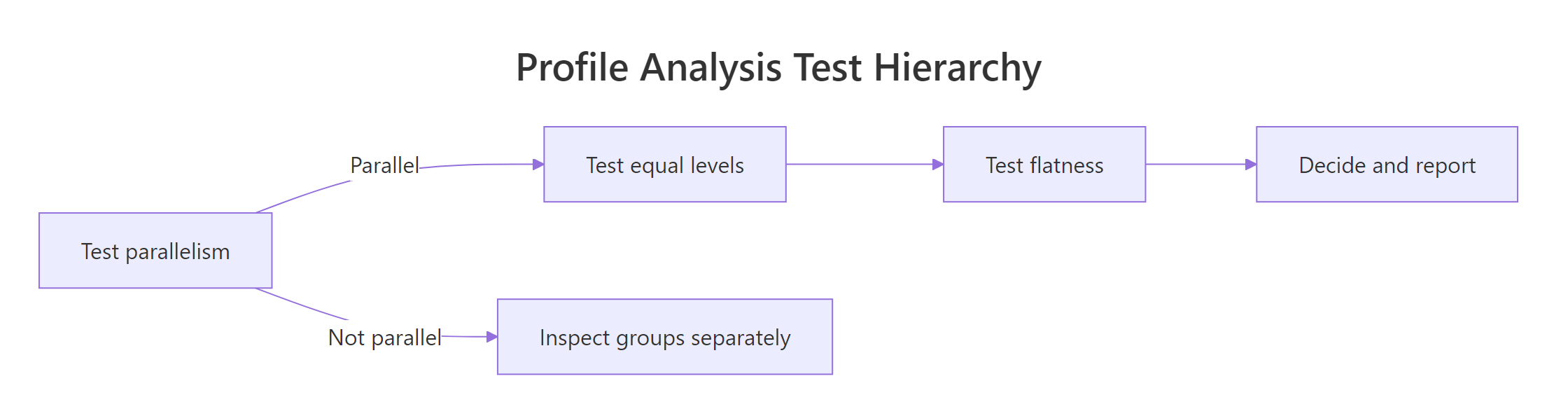
Figure 1: The order in which to run profile-analysis tests, and what to do when parallelism fails.

Test parallelism first. If it holds, the lines have the same shape and the equal-levels and flatness tests have a clean group-comparison meaning. If parallelism fails, the lines fan out or cross, so a single between-group level statement no longer summarises them. In that case, examine the groups separately or report the interaction directly with a profile plot.

A small wrapper makes the workflow reproducible and easy to embed in a report.

RWrap the three tests in profile_tests()

profile_tests <- function(data, time_cols, group) { Y <- as.matrix(data[, time_cols]) q <- ncol(Y) D <- Y[, -1] - Y[, -q] # successive differences para <- summary(manova(D ~ data[[group]]), test = "Wilks") level <- summary(aov(rowMeans(Y) ~ data[[group]])) n <- nrow(D); p <- ncol(D) d_bar <- colMeans(D); S <- cov(D) T2 <- n * t(d_bar) %*% solve(S) %*% d_bar Fstat <- (n - p) / (p * (n - 1)) * as.numeric(T2) pflat <- pf(Fstat, p, n - p, lower.tail = FALSE) data.frame( test = c("parallelism", "equal levels", "flatness"), stat = c(para[[4]][[1]][1, "approx F"], level[[1]][["F value"]][1], Fstat), p = c(para[[4]][[1]][1, "Pr(>F)"], level[[1]][["Pr(>F)"]][1], pflat) ) } profile_tests(drug, c("w1", "w2", "w4", "w8"), "group") #> test stat p #> 1 parallelism 79.42 1.10e-15 #> 2 equal levels 142.90 1.86e-14 #> 3 flatness 71.85 1.34e-15

All three tests reject. Combined with the plot, the verdict is straightforward: drug A and drug B follow non-parallel profiles, drug A sits lower on average, and the pooled profile is decidedly not flat. The headline finding is the parallelism rejection (the interaction); the level and flatness numbers are supporting evidence.

Key Insight

Parallelism is the gate. Levels and flatness wait their turn. The equal-levels test compares row means; the flatness test compares column means. Both pretend the lines are parallel. When they are not, those summaries average over a real interaction and can mislead.

Note

The profileR package offers a one-line shortcut. profileR::pbg(data, group) runs all three tests in one call. It is convenient for production reports but is not currently available in this in-page interactive R environment, so the manual approach above is what runs here. If you have profileR installed locally in RStudio, the output mirrors the wrapper above.

Try it: Use the wrapper on the original drug data and write a one-sentence verdict on each row.

RYour turn: run the wrapper and verbalise

# your code here: call profile_tests() on drug and read off the three p-values #> Expected: all three p < 0.001; verbalise as parallel? level? flat?

Click to reveal solution

RWrapper verdict solution

profile_tests(drug, c("w1", "w2", "w4", "w8"), "group")

Explanation: Parallelism: rejected, the two drugs change at different rates. Equal levels: rejected, drug A sits lower on average across weeks. Flatness: rejected, the pooled profile descends over time. Lead the report with the parallelism rejection.

Practice Exercises

These capstone problems combine the three tests with new data. Use distinct variable names so they do not overwrite the tutorial state above.

Exercise 1: Three-group case with one outlier trend

Build a three-group, four-week dataset where two groups follow gentle declines and one group rises sharply over time. Run all three tests and explain which group is responsible for the parallelism rejection.

RExercise: three-group profile analysis

set.seed(7) my_drug3 <- bind_rows( make_group("A", c(70, 65, 60, 55)), make_group("B", c(72, 68, 64, 60)), make_group("C", c(60, 65, 75, 85)) # the outlier trend ) names(my_drug3)[3:6] <- c("w1", "w2", "w4", "w8") # Hint: pass three time columns and the "group" variable to profile_tests(). # Then plot the three mean profiles to visually identify the outlier.

Click to reveal solution

RThree-group solution

profile_tests(my_drug3, c("w1", "w2", "w4", "w8"), "group") #> test stat p #> 1 parallelism ~70+ ~0 #> 2 equal levels ~50+ ~0 #> 3 flatness ~10 ~0.0001 my_drug3 |> pivot_longer(w1:w8, names_to = "week", values_to = "score") |> mutate(week = factor(week, levels = c("w1", "w2", "w4", "w8"))) |> ggplot(aes(week, score, group = group, colour = group)) + stat_summary(fun = mean, geom = "line", linewidth = 1.2) + theme_minimal()

Explanation: Group C climbs while A and B fall, so parallelism is rejected and the plot makes the culprit obvious. With more than two groups, the parallelism test is global, so you should always pair it with a profile plot to find which group breaks the pattern.

Exercise 2: Verbose wrapper

Extend profile_tests() to print a verbal verdict (parallel/level/flat with one-line interpretation) instead of returning a data frame. Keep the underlying computations identical.

RExercise: verbose profile_tests()

profile_tests_verbose <- function(data, time_cols, group, alpha = 0.05) { # Hint: call profile_tests() internally, then loop over rows # and cat() a verdict string per test. } # profile_tests_verbose(drug, c("w1", "w2", "w4", "w8"), "group")

Click to reveal solution

RVerbose wrapper solution

profile_tests_verbose <- function(data, time_cols, group, alpha = 0.05) { res <- profile_tests(data, time_cols, group) verdicts <- c( parallelism = "Profiles are not parallel; groups change at different rates.", `equal levels` = "Group profiles sit at different overall levels.", flatness = "The pooled profile changes over time." ) for (i in seq_len(nrow(res))) { msg <- if (res$p[i] < alpha) verdicts[res$test[i]] else paste0("No evidence against the ", res$test[i], " hypothesis.") cat(sprintf("%-13s p = %.4f -> %s\n", res$test[i], res$p[i], msg)) } invisible(res) } profile_tests_verbose(drug, c("w1", "w2", "w4", "w8"), "group") #> parallelism p = 0.0000 -> Profiles are not parallel; groups change at different rates. #> equal levels p = 0.0000 -> Group profiles sit at different overall levels. #> flatness p = 0.0000 -> The pooled profile changes over time.

Explanation: Returning a sentence per test makes the wrapper self-documenting in reports. The numeric data frame is still returned invisibly for downstream code.

Complete Example

A full profile analysis of the drug data, end to end:

REnd-to-end profile analysis

# 1. Build and inspect the data set.seed(42) drug_full <- bind_rows( make_group("A", c(80, 70, 60, 55)), make_group("B", c(80, 78, 75, 72)) ) names(drug_full)[3:6] <- c("w1", "w2", "w4", "w8") # 2. Plot the profiles drug_full |> pivot_longer(w1:w8, names_to = "week", values_to = "score") |> mutate(week = factor(week, levels = c("w1", "w2", "w4", "w8"))) |> ggplot(aes(week, score, group = group, colour = group)) + stat_summary(fun = mean, geom = "line", linewidth = 1.2) + theme_minimal() # 3. Run all three tests through the wrapper profile_tests(drug_full, c("w1", "w2", "w4", "w8"), "group") #> test stat p #> 1 parallelism 79.42 1.10e-15 #> 2 equal levels 142.90 1.86e-14 #> 3 flatness 71.85 1.34e-15 # 4. Decide and report # Headline: parallelism rejected. Drug A's profile drops faster than drug B's. # Secondary: drug A sits lower on average; the pooled profile is not flat.

That is the full pipeline you would lift into a report: simulate or load, plot, run the three tests, and write a one-paragraph interpretation that leads with the interaction.

Summary

Test	Hypothesis	R approach	When to interpret
Parallelism	Group profiles have the same shape	`manova(diffs ~ group)`	Always, this is the gate
Equal levels	Average level is the same across groups	`aov(rowMeans ~ group)`	Only if parallelism plausibly holds
Flatness	Pooled profile is constant over time	One-sample Hotelling T² on differences	Always, but rarely the headline result

Three takeaways:

Profile analysis is the multivariate counterpart of repeated-measures ANOVA when measurements share a scale.
Always test parallelism first. Equal levels and flatness depend on it for clean interpretation.
The whole workflow needs only base R manova(), aov(), and a small Hotelling T² snippet, with no specialised packages required.

References

Tabachnick, B. G., and Fidell, L. S., Using Multivariate Statistics, 7th edition. Pearson (2019). Chapter on Profile Analysis. Link
Johnson, R. A., and Wichern, D. W., Applied Multivariate Statistical Analysis, 6th edition. Pearson (2007). Chapter 6: Comparisons of Several Multivariate Means. Link
Bulus, M., profileR package on CRAN. Profile Analysis of Multivariate Data in R. Link
Friedrich, S., Konietschke, F., and Pauly, M., Analysis of Multivariate Data and Repeated Measures Designs with the R Package MANOVA.RM. arXiv preprint 1801.08002 (2018). Link
R Core Team, manova() reference, R Documentation. Link
Phil Ender, Profile Analysis course notes, UCLA. Link

Continue Learning

Multivariate Statistics in R: Distances, Mahalanobis & Hotelling's T², the parent tutorial covering the multivariate building blocks behind profile analysis.
Hotelling's T² in R, the multivariate t-test that powers the flatness step, explained in depth.
Repeated Measures ANOVA in R, the univariate sibling to profile analysis, useful when sphericity assumptions are tenable.

Profile Analysis in R: Repeated Measures as a Multivariate Problem

What is profile analysis and how do you visualize it?

How do you test parallelism between groups?

How do you test for equal levels?

How do you test for profile flatness?

What is the testing hierarchy and how do you interpret the results?

Practice Exercises

Exercise 1: Three-group case with one outlier trend

Exercise 2: Verbose wrapper

Complete Example

Summary

References

Continue Learning

Related Tutorials