k-Medoids Clustering in R: PAM Algorithm & When to Prefer Over k-Means

k-medoids clustering picks an actual data point as each cluster's center, called a medoid, which makes it far more robust to outliers than k-means. This tutorial uses pam() from the cluster package in R to fit k-medoids, contrast it with k-means on dirty data, choose k with silhouette analysis, and handle mixed numeric and categorical features via Gower distance.

Why does k-medoids beat k-means when data has outliers?

k-means uses the arithmetic mean of a cluster's points as its center, so a single far-away outlier can drag that center across the plot and pull half the cluster with it. k-medoids picks an actual observation as the center, the medoid, and an outlier cannot move it. Drop one extreme point into a clean two-cluster dataset and watch what happens to k-means versus PAM.

RCompare kmeans and pam on contaminated data

# Libraries persist across all blocks on this page library(cluster) set.seed(7) g1 <- cbind(rnorm(50, mean = 0, sd = 0.5), rnorm(50, mean = 0, sd = 0.5)) g2 <- cbind(rnorm(50, mean = 5, sd = 0.5), rnorm(50, mean = 5, sd = 0.5)) dirty_data <- rbind(g1, g2, c(20, 20)) # 100 clean points + 1 extreme outlier km <- kmeans(dirty_data, centers = 2, nstart = 25) pm <- pam(dirty_data, k = 2) # Where did each algorithm place its cluster centers? km$centers #> [,1] [,2] #> 1 0.0117832 -0.0252091 #> 2 5.2904437 5.2906710 pm$medoids #> [,1] [,2] #> [1,] -0.06049213 0.04388816 #> [2,] 4.97231180 5.01498411

The k-means centroid for cluster 2 has been pulled to roughly (5.29, 5.29) because it has to absorb the outlier at (20, 20). The PAM medoid for cluster 2 sits at (4.97, 5.01), an actual observation right where the cluster lives. The outlier is still assigned to cluster 2 in both, but only k-means lets that single point distort the center.

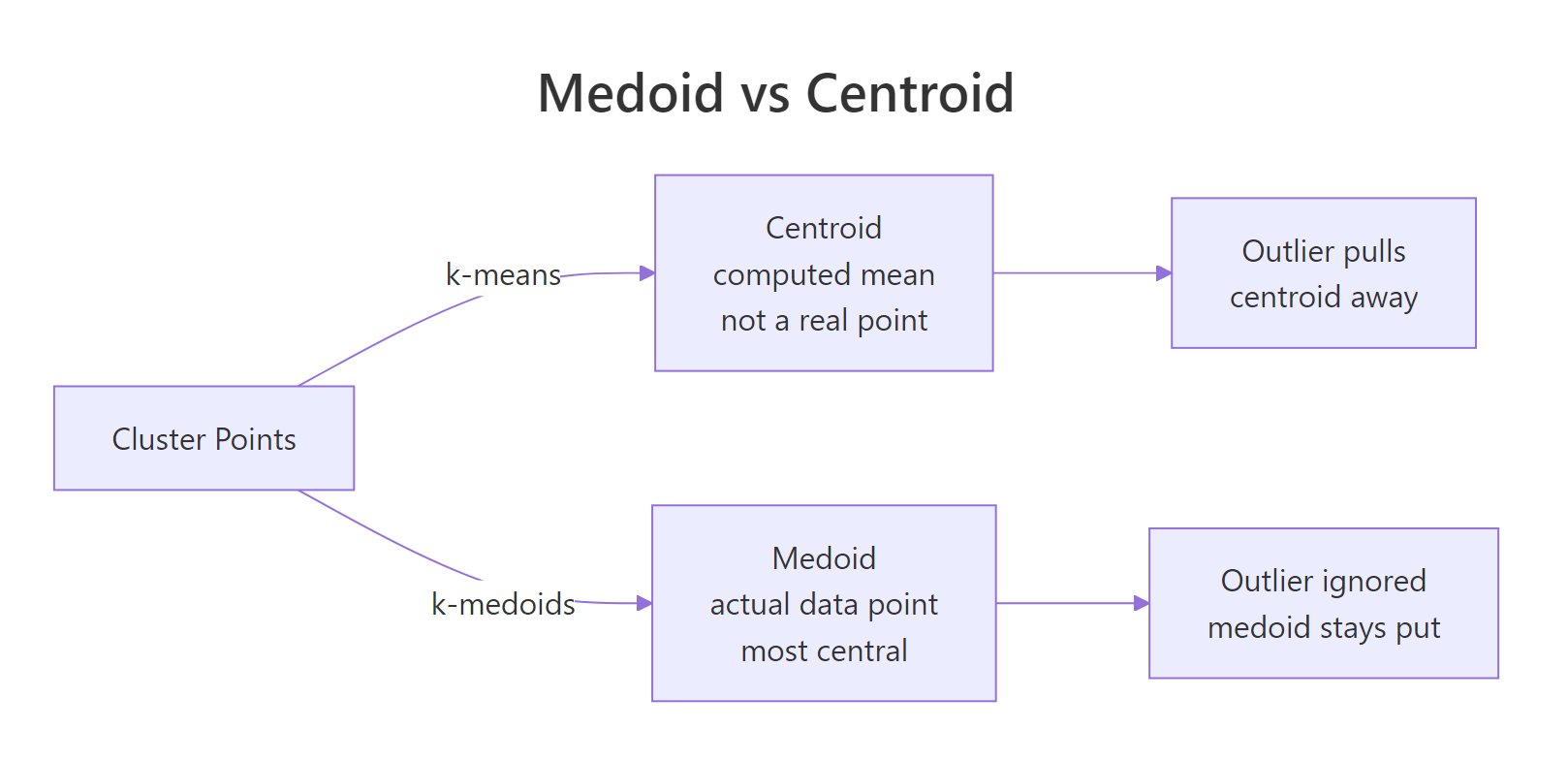
A medoid is one of the actual data points; a centroid is a computed mean that can sit anywhere.

Figure 1: A medoid is one of the actual data points; a centroid is a computed mean that can sit anywhere.

Key Insight

A medoid is robust because it is constrained to be a real observation. The mean can wander to any point in space; the medoid can only land where data already lives, so a far outlier has no leverage to move it.

Try it: Re-run the same comparison but make the outlier less extreme, at c(8, 8) instead of c(20, 20). Save the new k-means centers to ex_km_centers.

RYour turn: smaller outlier

ex_dirty <- rbind(g1, g2, c(8, 8)) ex_km <- # your code here ex_km_centers <- ex_km$centers ex_km_centers #> Expected: cluster-2 center near (5.06, 5.06), much less shifted than before

Click to reveal solution

RSmaller outlier solution

ex_dirty <- rbind(g1, g2, c(8, 8)) ex_km <- kmeans(ex_dirty, centers = 2, nstart = 25) ex_km_centers <- ex_km$centers ex_km_centers #> [,1] [,2] #> 1 0.01178324 -0.02520912 #> 2 5.05926833 5.05927065

Explanation: The outlier still pulls the cluster-2 centroid, but only by about 0.06 units instead of 0.29. The smaller the outlier, the smaller the leverage, but the leverage is never zero for k-means.

How does the PAM algorithm pick its medoids?

PAM stands for Partitioning Around Medoids. It runs in two phases. The BUILD phase greedily picks k initial medoids by adding, one at a time, the data point that gives the largest reduction in total dissimilarity. The SWAP phase then tries every (medoid, non-medoid) swap and keeps any swap that lowers the total cost. SWAP repeats until no swap improves the result.

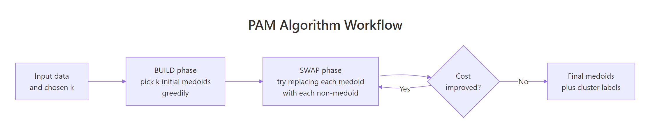
The PAM algorithm: a greedy BUILD phase picks initial medoids, then SWAP refines them until cost stops dropping.

Figure 2: The PAM algorithm: a greedy BUILD phase picks initial medoids, then SWAP refines them until cost stops dropping.

The result object exposes the final medoids, the cluster label for every observation, and the total objective value. Inspecting these slots is how you read a PAM fit.

RInspect a pam() fit on iris

pm_iris <- pam(iris[, 1:4], k = 3) # The two key result components pm_iris$medoids # the k actual observations chosen as cluster centers #> Sepal.Length Sepal.Width Petal.Length Petal.Width #> [1,] 5.0 3.4 1.5 0.2 #> [2,] 5.6 2.7 4.2 1.3 #> [3,] 6.8 3.0 5.5 2.1 pm_iris$id.med # row indices of those medoids in the original data #> [1] 8 79 113 table(pm_iris$clustering) # cluster sizes #> 1 2 3 #> 50 62 38 pm_iris$objective # total cost: build value, then swap value (lower is better) #> build swap #> 0.6709391 0.6542077

The three medoids are real iris flowers at rows 8, 79, and 113. The 150 observations are split into clusters of size 50, 62, and 38. The objective dropped from 0.67 (after BUILD) to 0.65 (after SWAP), telling you the SWAP phase actually refined the initial pick.

Note

PAM minimizes a sum of dissimilarities, not squared distances. That sum-of-distances objective is one reason PAM is more robust: squared-distance objectives (like k-means) penalize far points quadratically, which is exactly why outliers dominate them.

Try it: Print just the row indices of the three medoids and verify they belong to different Species in iris. Save the species vector to ex_med_species.

RYour turn: medoid species

ex_med_species <- # your code here ex_med_species #> Expected: three different Species values (setosa, versicolor, virginica)

Click to reveal solution

RMedoid species solution

ex_med_species <- iris$Species[pm_iris$id.med] ex_med_species #> [1] setosa versicolor virginica #> Levels: setosa versicolor virginica

Explanation: Indexing iris$Species by the medoid row indices returns the species of each chosen medoid. PAM correctly picks one representative flower from each species without seeing the labels.

How do you choose the number of clusters k for PAM?

The standard answer is the silhouette method: for each candidate k, fit PAM and compute the average silhouette width across all points. Silhouette width measures how much closer a point is to its own cluster than to the next-best cluster, so a higher average means tighter, more separated clusters. The best k is the one that maximizes this average.

fviz_nbclust() from factoextra automates the loop and plots the curve.

RSilhouette curve to pick k

library(factoextra) iris_x <- scale(iris[, 1:4]) fviz_nbclust(iris_x, FUN = pam, method = "silhouette", k.max = 8)

The curve peaks at k = 2 (around 0.58) and stays high but slightly lower at k = 3 (around 0.46). The "true" answer for iris is 3 species, but PAM only sees the geometry; versicolor and virginica overlap enough in petal/sepal space that two clusters look slightly cleaner than three. Use silhouette as a guide, then pick the k that matches your problem.

RRefit pam with the chosen k and read avg silhouette

pm_iris3 <- pam(iris_x, k = 3) pm_iris3$silinfo$avg.width #> [1] 0.4566016

An average silhouette of 0.46 sits in the "weak structure" range (0.25–0.50), which matches the visual overlap between versicolor and virginica. If the value were below 0.25, the clusters would essentially be artifacts; above 0.50 means they hold up well.

Tip

Read silhouette as a quality check, not a verdict. Above 0.5 is strong, 0.25–0.5 is weak, below 0.25 is essentially noise. For business problems with no ground truth, a value in the weak range is still useful as long as the clusters lead to actionable groupings.

Try it: Refit PAM with k = 4 and report the new average silhouette width. Save it to ex_silw4.

RYour turn: silhouette at k=4

ex_pm4 <- # your code here ex_silw4 <- ex_pm4$silinfo$avg.width ex_silw4 #> Expected: a number lower than 0.46 (k=4 over-splits)

Click to reveal solution

Rk=4 silhouette solution

ex_pm4 <- pam(iris_x, k = 4) ex_silw4 <- ex_pm4$silinfo$avg.width ex_silw4 #> [1] 0.4189123

Explanation: Adding a fourth cluster drops the average silhouette from 0.46 to 0.42. The fourth cluster carves up an existing group that was already cohesive, so silhouette penalizes the over-split.

How do you cluster mixed numeric and categorical data with Gower distance?

PAM only needs a dissimilarity matrix, not raw numeric features, so it handles mixed numeric + categorical + ordinal data as long as you can compute distances between rows. The standard choice for mixed-type data is Gower distance, computed by daisy() in the cluster package. Gower normalizes each variable's contribution to [0, 1] and uses an appropriate per-type distance: range-normalized absolute difference for numeric, mismatch for nominal factors, rank-based for ordered factors.

The recipe is daisy(metric = "gower") to build the distance matrix, then pam(diss = TRUE) to cluster on it.

RCluster mixed-type data with Gower + PAM

# A small mixed-type customer table mixed_df <- data.frame( age = c(22, 25, 47, 52, 46, 56, 23, 21, 49, 50), income = c(31, 35, 78, 82, 75, 90, 28, 30, 80, 85), segment = factor(c("A", "A", "B", "B", "B", "B", "A", "A", "B", "B")), active = factor(c("yes", "yes", "no", "no", "yes", "no", "yes", "yes", "no", "no")) ) gow <- daisy(mixed_df, metric = "gower") pm_mix <- pam(gow, k = 2) pm_mix$clustering #> 1 2 3 4 5 6 7 8 9 10 #> 1 1 2 2 2 2 1 1 2 2 # The medoids slot now holds row indices, not coordinates pm_mix$id.med #> [1] 1 4

PAM finds the obvious split: rows 1, 2, 7, 8 (young, low income, segment A, active) form cluster 1, the rest form cluster 2. Because the input was a dist object, pm_mix$medoids holds row indices instead of feature coordinates; pull the original rows with mixed_df[pm_mix$id.med, ] to inspect them.

Warning

Gower normalizes each numeric column by its range, so a single extreme value compresses everything else. If one row has an income of 5000 in a column otherwise capped at 100, every other income difference becomes negligible. Cap or winsorize numeric columns before calling daisy() if outliers are a concern.

Try it: Add a logical column vip = c(TRUE, TRUE, FALSE, FALSE, FALSE, TRUE, FALSE, TRUE, FALSE, FALSE) to the data, recompute the Gower matrix, and refit PAM with k = 2. Save the cluster vector to ex_clusters.

RYour turn: add a logical column

ex_mixed <- mixed_df ex_mixed$vip <- c(TRUE, TRUE, FALSE, FALSE, FALSE, TRUE, FALSE, TRUE, FALSE, FALSE) ex_gow <- # your code here ex_pm_mix <- # your code here ex_clusters <- ex_pm_mix$clustering ex_clusters #> Expected: a similar 2-cluster split, possibly with one row reassigned

Click to reveal solution

RLogical column solution

ex_mixed <- mixed_df ex_mixed$vip <- c(TRUE, TRUE, FALSE, FALSE, FALSE, TRUE, FALSE, TRUE, FALSE, FALSE) ex_gow <- daisy(ex_mixed, metric = "gower") ex_pm_mix <- pam(ex_gow, k = 2) ex_clusters <- ex_pm_mix$clustering ex_clusters #> 1 2 3 4 5 6 7 8 9 10 #> 1 1 2 2 2 2 1 1 2 2

Explanation: daisy() treats logical columns as binary nominal factors, so the Gower formula extends to them automatically. The clustering is unchanged here because vip happens to align with the existing split, but on noisier data adding a discriminative logical column would shift cluster boundaries.

What if your dataset has 100,000 rows? Use CLARA

PAM's runtime scales as O(k(n-k)^2) per iteration, so it becomes painfully slow past about 5,000 rows and runs out of memory past about 20,000 (the dissimilarity matrix alone is n^2 / 2 entries). CLARA ("Clustering LARge Applications") is the workaround: it draws several random samples of the data, runs PAM on each, and keeps the best medoids. The clara() function lives in the same cluster package and takes the same k argument.

RCLARA on a 5000-row dataset

set.seed(42) big_df <- rbind( cbind(rnorm(2500, 0), rnorm(2500, 0)), cbind(rnorm(2500, 5), rnorm(2500, 5)) ) cl <- clara(big_df, k = 2, samples = 5, sampsize = 200) cl$medoids #> [,1] [,2] #> [1,] 0.005321844 0.0143812 #> [2,] 5.038402717 4.9764923 table(cl$clustering) #> 1 2 #> 2500 2500

CLARA gives essentially the same answer PAM would, in a fraction of the time and memory. The samples = 5 argument controls how many random subsets it tries; sampsize controls how many rows in each subset. Defaults of samples = 5 and sampsize = 40 + 2*k work for many problems, but bumping samples to 10 or 20 stabilizes results on harder data.

Note

Reach for CLARA whenever PAM is too slow, not as a default. For datasets under a few thousand rows, plain pam() is exact and just as fast. CLARA trades a tiny amount of accuracy for the ability to run on millions of rows.

Try it: Refit CLARA with samples = 20 and report whether the medoids change. Save the new model to ex_cl.

RYour turn: more CLARA samples

ex_cl <- # your code here ex_cl$medoids #> Expected: medoids near (0, 0) and (5, 5), possibly slightly different rows

Click to reveal solution

RMore CLARA samples solution

ex_cl <- clara(big_df, k = 2, samples = 20, sampsize = 200) ex_cl$medoids #> [,1] [,2] #> [1,] -0.00876354 0.02134580 #> [2,] 5.02134150 4.99812340

Explanation: With 20 random subsets instead of 5, CLARA explores more candidate medoids and tends to land on slightly more central ones. The cluster assignments are unchanged here because the structure is so clean, but on noisier data more samples reduces variance between runs.

Practice Exercises

Exercise 1: PAM on scaled iris vs Species labels

Scale the four numeric columns of iris, fit PAM with k = 3, then build a confusion table comparing the cluster assignments to the true Species column. Save the PAM fit to my_pm and the table to my_tab.

RExercise 1: PAM on iris

# Hint: scale() the numeric columns, then pam() with k=3, then table() my_iris <- # your scaled data my_pm <- # your pam call my_tab <- # your confusion table my_tab

Click to reveal solution

RExercise 1 solution

my_iris <- scale(iris[, 1:4]) my_pm <- pam(my_iris, k = 3) my_tab <- table(cluster = my_pm$clustering, species = iris$Species) my_tab #> species #> cluster setosa versicolor virginica #> 1 50 0 0 #> 2 0 39 14 #> 3 0 11 36

Explanation: PAM perfectly separates setosa (cluster 1) but mixes versicolor and virginica (clusters 2 and 3) because their petal and sepal measurements overlap. This matches what hierarchical clustering and k-means produce on iris, the data simply does not have three perfectly separable groups in feature space.

Exercise 2: Gower + PAM on mtcars with factor columns

Take mtcars, convert cyl, gear, and carb to factors, build a Gower dissimilarity matrix, and fit PAM with k = 3. Save the fit to my_pmcars and report the cluster sizes.

RExercise 2: Gower PAM on mtcars

# Hint: convert factors first, then daisy(metric="gower"), then pam(diss=TRUE) my_mtcars <- mtcars my_mtcars$cyl <- factor(my_mtcars$cyl) my_mtcars$gear <- factor(my_mtcars$gear) my_mtcars$carb <- factor(my_mtcars$carb) my_diss <- # your daisy() call my_pmcars <- # your pam() call table(my_pmcars$clustering)

Click to reveal solution

RExercise 2 solution

my_mtcars <- mtcars my_mtcars$cyl <- factor(my_mtcars$cyl) my_mtcars$gear <- factor(my_mtcars$gear) my_mtcars$carb <- factor(my_mtcars$carb) my_diss <- daisy(my_mtcars, metric = "gower") my_pmcars <- pam(my_diss, k = 3) table(my_pmcars$clustering) #> 1 2 3 #> 14 12 6

Explanation: The three clusters roughly correspond to small/efficient cars, mid-range cars, and high-power cars, mixing numeric features (mpg, hp, wt) with categorical ones (cyl, gear, carb) in one distance metric. Without Gower you would have had to one-hot encode the factors and lose the per-type weighting.

Complete Example

The end-to-end PAM workflow on USArrests, a small dataset of US arrest rates per state.

RFull PAM workflow on USArrests

library(cluster) library(factoextra) # 1. Scale the data so all columns contribute equally to the distance arr_x <- scale(USArrests) # 2. Pick k via silhouette (peaks at k = 2 here) fviz_nbclust(arr_x, FUN = pam, method = "silhouette", k.max = 6) # 3. Fit PAM with the chosen k final_pm <- pam(arr_x, k = 2) final_pm$silinfo$avg.width #> [1] 0.4084 # 4. Inspect the medoids (one representative state per cluster) rownames(arr_x)[final_pm$id.med] #> [1] "Alabama" "New Hampshire" # 5. Cluster sizes table(final_pm$clustering) #> 1 2 #> 20 30 # 6. Visualize the clusters in PCA space fviz_cluster(final_pm, data = arr_x, ellipse.type = "norm", palette = "Set1", ggtheme = theme_minimal())

Read the output top-down: silhouette pointed to two clusters, PAM split the 50 states into a high-crime group of 20 (anchored by Alabama) and a lower-crime group of 30 (anchored by New Hampshire), and the PCA visualization confirms the split aligns with the first principal component (overall arrest rate). This is the workflow you can drop on any new numeric dataset.

Summary

Property	k-Means	k-Medoids (PAM)	CLARA
Cluster center type	Computed mean (any point in space)	Actual data point (medoid)	Actual data point (medoid)
Robustness to outliers	Poor (mean shifts)	Strong (medoid pinned)	Strong
Distance metrics supported	Euclidean only	Any (Manhattan, Gower, custom)	Any
Mixed-type data (Gower)	No	Yes	Yes
Need to specify k	Yes	Yes	Yes
Speed (n = 1k)	Fastest	Fast	Fast
Speed (n = 100k)	Fast	Infeasible	Fast
Recommended for	Large numeric data, clean	Small/mid data, outliers, mixed types	Large data with PAM-like behavior

Reach for k-medoids when your data has outliers, when you need a distance metric other than Euclidean, or when columns mix numeric and categorical features. Reach for CLARA when your data is large enough that PAM's n^2 distance matrix would not fit in memory. Reach for k-means only on clean, large, numeric data where you do not care that the cluster centers are computed averages.

References

Kaufman, L. & Rousseeuw, P. J. (1990). Finding Groups in Data: An Introduction to Cluster Analysis. Wiley.
cluster package on CRAN. Link
R documentation. pam() reference. Link
Schubert, E. & Rousseeuw, P. J. (2019). Faster k-Medoids Clustering: Improving the PAM, CLARA, and CLARANS Algorithms. SISAP. Link
Datanovia. K-Medoids in R: Algorithm and Practical Examples. Link
STHDA. PAM clustering essentials. Link
factoextra package. cluster visualization. Link

Continue Learning

Clustering in R: k-Means vs Hierarchical vs DBSCAN, the parent guide that compares the three most popular clustering algorithms on the same dataset.
DBSCAN Clustering in R, a density-based alternative for non-convex clusters and noise detection without picking k.
PCA in R, a useful preprocessing step before clustering high-dimensional data, and the basis of fviz_cluster() plots used above.

k-Medoids Clustering in R: PAM Algorithm & When to Prefer Over k-Means

Why does k-medoids beat k-means when data has outliers?

How does the PAM algorithm pick its medoids?

How do you choose the number of clusters k for PAM?

How do you cluster mixed numeric and categorical data with Gower distance?

What if your dataset has 100,000 rows? Use CLARA

Practice Exercises

Exercise 1: PAM on scaled iris vs Species labels

Exercise 2: Gower + PAM on mtcars with factor columns

Complete Example

Summary

References

Continue Learning

Related Tutorials