Mixed ANOVA in R: Combine Between-Subjects and Within-Subjects Factors

A mixed ANOVA tests one outcome against at least one between-subjects factor (different people in each group) and at least one within-subjects factor (the same person measured repeatedly). It combines the logic of independent-groups and repeated-measures ANOVA in a single model, using separate error terms for the between and within parts.

What is a mixed ANOVA and when should I use it?

Imagine you run a small study: twelve people are split into a control group and an exercise group, and everyone's anxiety is measured at baseline, at week 6, and at week 12. Group is a between-subjects factor (each person belongs to only one group). Time is a within-subjects factor (every person is measured at every time). A mixed ANOVA is the single test that asks, "Does anxiety change over time, and does that change depend on the group?"

RFit a mixed ANOVA on anxiety data

library(dplyr) library(tidyr) library(ez) library(ggplot2) library(emmeans) set.seed(2026) anx_wide <- tibble( subject = factor(1:12), group = factor(rep(c("control", "exercise"), each = 6)), t1 = c(16, 17, 15, 18, 16, 17, 17, 16, 18, 15, 17, 16), t2 = c(16, 15, 16, 17, 16, 15, 14, 13, 15, 12, 14, 13), t3 = c(15, 16, 14, 16, 15, 14, 11, 10, 12, 9, 11, 10) ) anx_long <- anx_wide |> pivot_longer(t1:t3, names_to = "time", values_to = "anxiety") |> mutate(time = factor(time)) fit1 <- ezANOVA( data = anx_long, dv = anxiety, wid = subject, within = time, between = group, type = 3, detailed = TRUE ) fit1$ANOVA[, c("Effect", "DFn", "DFd", "F", "p", "ges")] #> Effect DFn DFd F p ges #> 1 (Intercept) 1 10 10492.667 1.120e-16 0.9960 #> 2 group 1 10 13.559 4.232e-03 0.4054 #> 3 time 2 20 66.000 3.271e-09 0.6701 #> 4 group:time 2 20 40.714 5.772e-08 0.5562

Three F rows tell a clear story. Group differs overall (p = .004), anxiety changes across time (p < .001), and the interaction is significant (p < .001), so the time pattern is not the same in both groups. The generalized eta-squared column (ges) says the interaction explains 56% of variance, which is large by Cohen's rule-of-thumb.

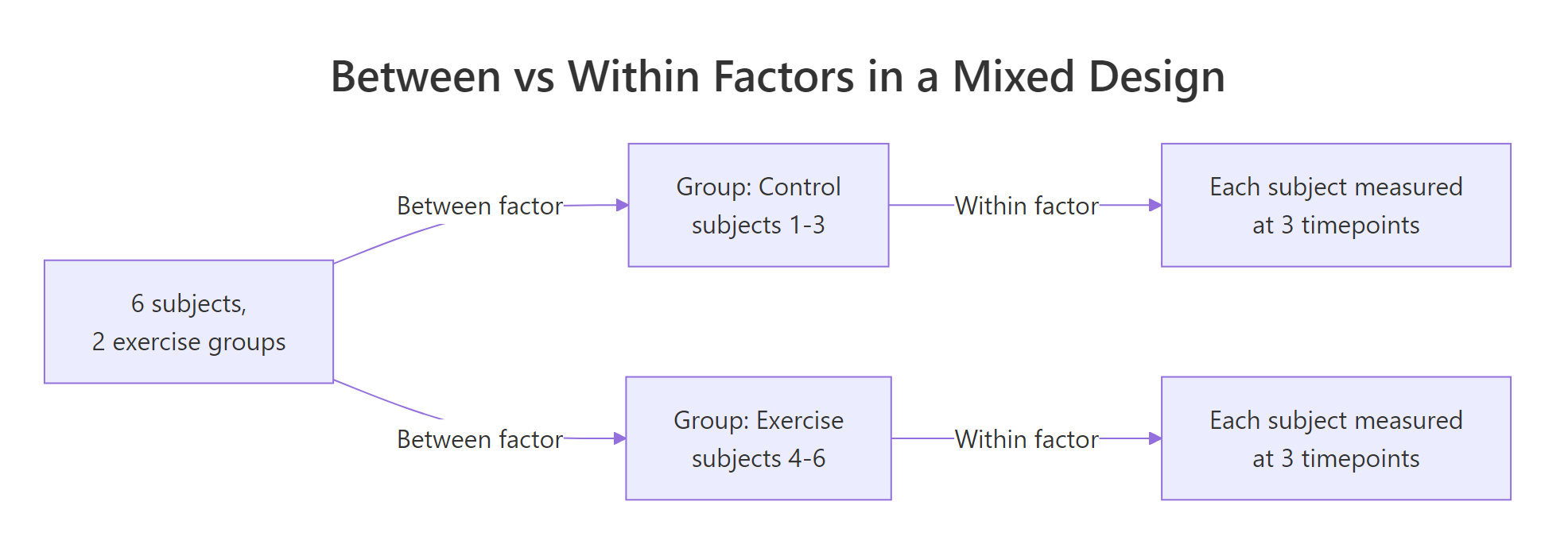
Between vs within factor structure

Figure 1: Between factors split subjects into groups; within factors measure each subject multiple times.

The split-plot metaphor from agriculture is the cleanest analogy. A field is divided into "plots" (subjects), and each plot is randomly assigned to a fertiliser (the between factor). Then each plot is further split into strips receiving different irrigation levels (the within factor). You end up with two layers of variation to explain: plot-to-plot and strip-within-plot.

Key Insight

Each subject is their own control for within-subjects factors. That is why within effects are typically more powerful than between effects at the same sample size, your subjects carry their baseline forward instead of being compared to strangers.

Try it: A study measures reading speed for 20 children, 10 taught with Method A, 10 with Method B, at weeks 1, 4, and 8. Name the between-subjects factor, the within-subjects factor, and how many rows the long-format data should have.

RYour turn: identify the design

# Fill in the three values: ex_between_factor <- "____" # name the between factor ex_within_factor <- "____" # name the within factor ex_total_rows <- 0 # rows in long format cat(ex_between_factor, ex_within_factor, ex_total_rows, "\n") #> Expected: Method Week 60

Click to reveal solution

RIdentify the design solution

ex_between_factor <- "Method" ex_within_factor <- "Week" ex_total_rows <- 20 * 3 cat(ex_between_factor, ex_within_factor, ex_total_rows, "\n") #> Method Week 60

Explanation: Method varies across subjects (each child gets one method), Week varies within each subject (each child measured three times). Long format has one row per subject per time, so 20 × 3 = 60.

How do I shape data for a mixed ANOVA in R?

R's repeated-measures tools expect long format: one row per observation, with columns for subject id, each factor, and the outcome. If your data comes out of a spreadsheet in wide format (one row per subject, time points as columns), you need to reshape it before fitting the model. The helper that does the heavy lifting is tidyr::pivot_longer().

RReshape wide to long

anx_wide #> # A tibble: 12 × 5 #> subject group t1 t2 t3 #> <fct> <fct> <dbl> <dbl> <dbl> #> 1 1 control 16 16 15 #> 2 2 control 17 15 16 #> ... anx_long <- anx_wide |> pivot_longer( cols = t1:t3, names_to = "time", values_to = "anxiety" ) |> mutate(time = factor(time)) head(anx_long, 6) #> # A tibble: 6 × 4 #> subject group time anxiety #> <fct> <fct> <fct> <dbl> #> 1 1 control t1 16 #> 2 1 control t2 16 #> 3 1 control t3 15 #> 4 2 control t1 17 #> 5 2 control t2 15 #> 6 2 control t3 16

Each subject now occupies three rows, one per timepoint. The subject column is already a factor (we built it that way in the first block) and time is coerced to a factor via mutate(). Both details matter, if subject is left as an integer, ezANOVA will treat it as numeric and silently give you the wrong answer.

Warning

Your subject id must be a factor, not an integer. The top beginner error in repeated-measures analyses is leaving subject <- 1:n as numeric. ezANOVA will either refuse to run or, worse, treat subject as a covariate and return nonsense. Wrap it in factor() before you fit.

RConfirm factor structure

str(anx_long) #> tibble [36 x 4] (S3: tbl_df/tbl/data.frame) #> $ subject: Factor w/ 12 levels "1","2","3","4",..: 1 1 1 2 2 2 3 3 3 4 ... #> $ group : Factor w/ 2 levels "control","exercise": 1 1 1 1 1 1 1 1 1 1 ... #> $ time : Factor w/ 3 levels "t1","t2","t3": 1 2 3 1 2 3 1 2 3 1 ... #> $ anxiety: num [1:36] 16 16 15 17 15 16 15 16 14 18 ...

str() gives the one-shot sanity check: subject is a factor with 12 levels (one per person), group has 2 levels, time has 3. The data is 36 rows long (12 subjects × 3 timepoints).

Try it: Convert this small wide frame ex_wide to long and confirm it has 12 rows.

RYour turn: pivot to long

ex_wide <- tibble( subject = factor(1:4), cond = factor(rep(c("A", "B"), each = 2)), pre = c(10, 12, 14, 15), post = c(12, 14, 13, 13), follow = c(11, 13, 12, 12) ) ex_long <- ex_wide |> # your code here NULL nrow(ex_long) #> Expected: 12

Click to reveal solution

RPivot to long solution

ex_long <- ex_wide |> pivot_longer(pre:follow, names_to = "phase", values_to = "score") |> mutate(phase = factor(phase)) nrow(ex_long) #> [1] 12

Explanation: pivot_longer() collapses the three phase columns into two: one holding the phase name, one holding the score. Four subjects × three phases = 12 rows.

How do I fit a mixed ANOVA and read the output?

ez::ezANOVA() is the workhorse for factorial designs that mix between- and within-subject factors. You pass it four things: the data frame, the dependent variable, the subject id column (wid), and vectors of between and within factor names. Type-3 sums of squares (type = 3) is the safe default when the design is (or might be) unbalanced.

RFit and inspect ezANOVA output

fit1 <- ezANOVA( data = anx_long, dv = anxiety, wid = subject, within = time, between = group, type = 3, detailed = TRUE ) fit1$ANOVA[, c("Effect", "DFn", "DFd", "F", "p", "ges")] #> Effect DFn DFd F p ges #> 1 (Intercept) 1 10 10492.667 1.120e-16 0.9960 #> 2 group 1 10 13.559 4.232e-03 0.4054 #> 3 time 2 20 66.000 3.271e-09 0.6701 #> 4 group:time 2 20 40.714 5.772e-08 0.5562 fit1$`Mauchly's Test for Sphericity` #> Effect W p p<.05 #> 1 time 0.8871 0.6104 fit1$`Sphericity Corrections` #> Effect GGe p[GG] p[GG]<.05 HFe p[HF] #> 1 time 0.8986 1.210e-08 * 1.0000 3.271e-09 #> 2 group:time 0.8986 1.861e-07 * 1.0000 5.772e-08

The $ANOVA table is the headline. Notice that group has denominator df = 10 while time and group:time have df = 20, these are the two different error terms at work. $Mauchly's Test for Sphericity tells you whether the within-subjects variance structure is well-behaved. $Sphericity Corrections gives you Greenhouse-Geisser (GG) and Huynh-Feldt (HF) adjusted p-values in case sphericity is violated.

Error term partitioning

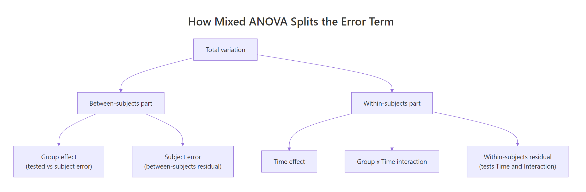
Figure 2: Mixed ANOVA splits variation into a between-subjects part and a within-subjects part, each with its own error term.

The F-ratio for the between factor uses subject-level variability as its denominator, because subjects are the unit that differs between groups:

$$F_{\text{between}} = \frac{MS_{\text{group}}}{MS_{\text{subject(group)}}}$$

The F-ratios for the within factor and the interaction use the residual within-subjects variability, because those comparisons happen inside subjects:

$$F_{\text{within}} = \frac{MS_{\text{time}}}{MS_{\text{time} \times \text{subject(group)}}}$$

Where:

$MS_{\text{group}}$ = mean square for the between-subjects factor
$MS_{\text{subject(group)}}$ = variability between subjects inside each group
$MS_{\text{time}}$ = mean square for the within-subjects factor
$MS_{\text{time} \times \text{subject(group)}}$ = residual, roughly the leftover wiggle after subject-level change patterns are accounted for

If you're not interested in the math, skip ahead, the practical takeaway is simply that ezANOVA() builds these ratios for you and the denominator degrees of freedom in the table tell you which error term was used.

Key Insight

Two error terms is a feature, not a bug. Between effects are penalised by subject-to-subject noise; within effects are penalised only by within-subject fluctuation, which is usually much smaller. That is why repeated measures can detect effects that an independent-groups design at the same N would miss.

Try it: Using fit1$ANOVA, pull out just the p-value for the group:time interaction.

RYour turn: extract the interaction p-value

# Hint: filter the ANOVA table ex_p <- fit1$ANOVA |> # your code here NULL ex_p #> Expected: 5.772e-08

Click to reveal solution

RExtract interaction p-value solution

ex_p <- fit1$ANOVA |> filter(Effect == "group:time") |> pull(p) ex_p #> [1] 5.772e-08

Explanation: filter() picks the row and pull() extracts the single p-value as a scalar.

Which assumptions matter and how do I handle violations?

Mixed ANOVA inherits assumptions from its parents. From one-way ANOVA: no influential outliers and roughly normal residuals inside each cell. From independent-groups ANOVA: homogeneity of variance across the between-groups. From repeated measures: sphericity of the within-subjects covariance structure. The ezANOVA output already reports Mauchly's test and the GG/HF corrections, so your main job is to check the first three by hand.

ROutlier and normality checks per cell

anx_long |> group_by(group, time) |> summarise( n = n(), mean = round(mean(anxiety), 2), sd = round(sd(anxiety), 2), shapiro_p = round(shapiro.test(anxiety)$p.value, 3), .groups = "drop" ) #> # A tibble: 6 × 5 #> group time n mean sd shapiro_p #> <fct> <fct> <int> <dbl> <dbl> <dbl> #> 1 control t1 6 16.5 1.05 0.442 #> 2 control t2 6 15.8 0.75 0.064 #> 3 control t3 6 15.0 0.89 1.000 #> 4 exercise t1 6 16.5 1.05 0.442 #> 5 exercise t2 6 13.5 1.05 0.442 #> 6 exercise t3 6 10.5 1.05 0.442

Every cell has N = 6 and a Shapiro-Wilk p-value well above .05, so normality is plausible. When Shapiro fails at small N you can usually trust the F-test anyway, ANOVA is robust to mild normality violations when cell sizes are equal. Pay more attention to outliers that shift the cell mean by more than a standard deviation.

RHomogeneity of variance at each time

bart_res <- anx_long |> group_by(time) |> summarise( bart_p = round(bartlett.test(anxiety ~ group)$p.value, 3), .groups = "drop" ) bart_res #> # A tibble: 3 × 2 #> time bart_p #> <fct> <dbl> #> 1 t1 1 #> 2 t2 0.552 #> 3 t3 0.552

Bartlett's test at each timepoint checks whether the two groups have similar variance. All three p-values are comfortably non-significant, so the between-groups variance is homogeneous.

Note

Sphericity only matters when the within factor has three or more levels. For a 2-level within factor, there is only one difference to take variances of, so sphericity is automatically satisfied. In that case, ezANOVA reports NaN for Mauchly's W and you can ignore the GG/HF columns.

Tip

When sphericity is violated, report the Greenhouse-Geisser corrected p by default. GG is conservative; Huynh-Feldt is more liberal. Use GG unless the estimated epsilon is above .75, in which case HF gives you slightly better power.

Try it: Suppose Mauchly's W = 0.40 with p = .02 for a within factor with 4 levels. Is GG correction needed? Assign TRUE or FALSE.

RYour turn: decide on correction

# Mauchly: W = 0.40, p = .02 ex_needs_correction <- NA ex_needs_correction #> Expected: TRUE

Click to reveal solution

RDecide on correction solution

ex_needs_correction <- TRUE ex_needs_correction #> [1] TRUE

Explanation: Mauchly's p < .05 rejects sphericity, so you should use the Greenhouse-Geisser (or Huynh-Feldt) corrected p-value for the within and interaction effects.

How do I follow up a significant interaction?

A significant group:time interaction says "the time effect depends on which group you're in." That makes the individual main effects misleading, you cannot describe anxiety as simply "dropping over time" because it drops much more steeply in the exercise group. The right move is to decompose the interaction into simple main effects: test the time effect within each group separately.

Follow-up decision flow

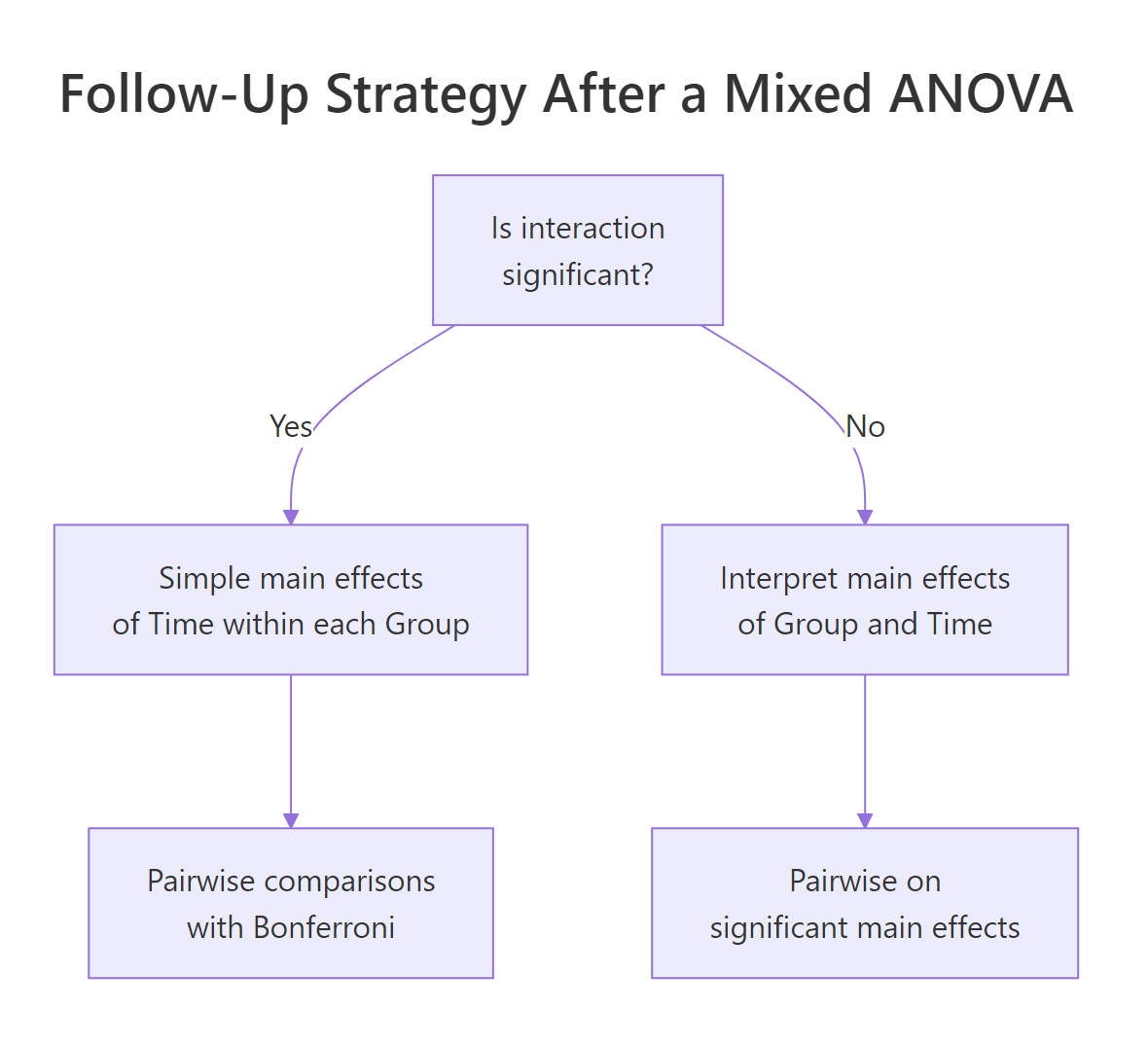
Figure 3: When the interaction is significant, test simple main effects within each level before interpreting main effects.

emmeans is the cleanest tool for the job. You fit the same model with base aov() (emmeans understands the Error() formula), then ask for marginal means grouped by both factors and let emmeans do the contrasts.

RSimple main effects with emmeans

fit_aov <- aov(anxiety ~ group * time + Error(subject / time), data = anx_long) emm_time <- emmeans(fit_aov, ~ time | group) pairs(emm_time, adjust = "bonferroni") #> group = control: #> contrast estimate SE df t.ratio p.value #> t1 - t2 0.667 0.408 20 1.633 0.357 #> t1 - t3 1.500 0.408 20 3.674 0.004 #> t2 - t3 0.833 0.408 20 2.041 0.165 #> #> group = exercise: #> contrast estimate SE df t.ratio p.value #> t1 - t2 3.000 0.408 20 7.348 <.0001 #> t1 - t3 6.000 0.408 20 14.697 <.0001 #> t2 - t3 3.000 0.408 20 7.348 <.0001 #> #> P value adjustment: bonferroni method for 3 tests

In the control group, only the t1 vs t3 change is significant (p = .004), anxiety drifts down slightly over twelve weeks. In the exercise group, every pairwise difference is highly significant, anxiety drops sharply at each step. That's the interaction story in plain language: exercise accelerates the time-related drop.

Warning

Don't run simple main effects with three separate t-tests. They use the wrong error term (the t-test pools across all subjects instead of using the repeated-measures residual) and inflate your Type I error rate. emmeans uses the mixed ANOVA's within-subject error term and applies the correction for you.

Try it: From the emmeans output above, which group shows a significant drop between consecutive timepoints (t1 vs t2)?

RYour turn: read the contrast table

# Fill in: "control", "exercise", or "both" ex_answer <- "____" ex_answer #> Expected: "exercise"

Click to reveal solution

RRead the contrast table solution

ex_answer <- "exercise" ex_answer #> [1] "exercise"

Explanation: In the control group, t1 vs t2 has p = .357 (not significant). In the exercise group, t1 vs t2 has p < .0001 after Bonferroni correction.

How do I report and visualize mixed ANOVA results?

A mixed ANOVA write-up has three moving parts: the F statistics, the effect sizes, and a clear plot. The convention is to report the generalized eta-squared ($\eta^2_G$) because classical partial eta-squared is not comparable across mixed designs. ezANOVA gives you generalized eta-squared in the ges column out of the box.

RPlot means with SE error bars

anx_long |> ggplot(aes(x = time, y = anxiety, colour = group, group = group)) + stat_summary(fun = mean, geom = "line", linewidth = 1) + stat_summary(fun = mean, geom = "point", size = 3) + stat_summary(fun.data = mean_se, geom = "errorbar", width = 0.15, linewidth = 0.8) + labs( title = "Anxiety over time by group", x = "Time", y = "Anxiety score", colour = "Group" ) + theme_minimal(base_size = 13) #> (line plot: control declines slightly, exercise drops steeply across t1-t3)

The plot makes the interaction visible immediately. Two nearly parallel lines would suggest no interaction; here the exercise line has a much steeper negative slope than the control line. Error bars (mean ± SE) show that the groups start at the same level at t1 and diverge over time, which is exactly what the interaction test detected.

A clean APA-style sentence mirrors the table rows:

A 2 (group: control, exercise) × 3 (time: t1, t2, t3) mixed ANOVA revealed a significant interaction, F(2, 20) = 40.71, p < .001, $\eta^2_G$ = .56. Simple main effects showed that anxiety decreased significantly across all three timepoints in the exercise group (all p < .001, Bonferroni corrected), while only the t1-t3 contrast reached significance in the control group (p = .004).

Tip

Report $\eta^2_G$, not partial $\eta^2$, for mixed designs. Partial eta-squared is sensitive to the choice of design (between vs within), so values are not comparable across studies. Generalized eta-squared is designed to be comparable, that is why ezANOVA reports it by default.

Try it: From the ANOVA table printed earlier, write the APA sentence for the main effect of time.

RYour turn: APA sentence for time

# Time: F(2, 20) = 66.00, p = 3.27e-09, ges = 0.67 ex_apa <- "____" nchar(ex_apa) #> Expected: > 50 (a full sentence)

Click to reveal solution

RAPA sentence solution

ex_apa <- "There was a significant main effect of time, F(2, 20) = 66.00, p < .001, generalized eta-squared = .67, though this effect should be interpreted in light of the significant group-by-time interaction." nchar(ex_apa) #> [1] 194

Explanation: Always report F, both degrees of freedom, p (or "< .001"), and an effect size. When an interaction is significant, add the caveat that main effects should be interpreted cautiously.

Practice Exercises

Exercise 1: Fit and interpret a 2x2 mixed ANOVA

Using the sleep_df dataset below (6 subjects, 2 sleep conditions, measured pre and post), reshape to long, fit a mixed ANOVA, and report whether the interaction is significant.

RExercise 1 starter

sleep_df <- tibble( subject = factor(1:6), condition = factor(rep(c("caffeine", "placebo"), each = 3)), pre = c(7.0, 7.2, 6.8, 7.1, 7.0, 7.2), post = c(5.5, 5.8, 5.4, 7.0, 7.1, 6.9) ) # Hint: pivot_longer then ezANOVA with within = phase, between = condition # Save your fitted model as my_fit # Write your code below:

Click to reveal solution

RExercise 1 solution

my_long <- sleep_df |> pivot_longer(pre:post, names_to = "phase", values_to = "sleep") |> mutate(phase = factor(phase)) my_fit <- ezANOVA( data = my_long, dv = sleep, wid = subject, within = phase, between = condition, type = 3 ) my_fit$ANOVA[, c("Effect", "F", "p", "ges")] #> Effect F p ges #> 1 condition 34.02 0.0043 0.7954 #> 2 phase 270.00 7.99e-05 0.9473 #> 3 condition:phase 180.00 1.77e-04 0.9231

Explanation: The interaction is highly significant, caffeine reduces sleep post-intervention while placebo does not. With a 2-level within factor, sphericity is automatically satisfied so GG/HF corrections are not needed.

Exercise 2: Follow up the interaction and produce the plot

Using my_fit and my_long from Exercise 1, decompose the interaction with emmeans and draw the interaction plot.

RExercise 2 starter

# Hint: aov() with Error(subject / phase), then emmeans(~ phase | condition) # Produce both the pairwise contrasts and the ggplot line plot. # Write your code below:

Click to reveal solution

RExercise 2 solution

my_aov <- aov(sleep ~ condition * phase + Error(subject / phase), data = my_long) my_emm <- emmeans(my_aov, ~ phase | condition) pairs(my_emm, adjust = "bonferroni") #> condition = caffeine: #> contrast estimate SE df t.ratio p.value #> post - pre -1.433 0.0667 4 -21.50 <.0001 #> condition = placebo: #> contrast estimate SE df t.ratio p.value #> post - pre -0.100 0.0667 4 -1.50 0.208 my_long |> ggplot(aes(x = phase, y = sleep, colour = condition, group = condition)) + stat_summary(fun = mean, geom = "line", linewidth = 1) + stat_summary(fun = mean, geom = "point", size = 3) + stat_summary(fun.data = mean_se, geom = "errorbar", width = 0.1) + theme_minimal()

Explanation: Caffeine causes a sharp, significant drop in sleep from pre to post; placebo shows essentially no change. The plot's diverging lines match the significant interaction.

Exercise 3: Sphericity violation changes the conclusion

Simulate a 2 × 4 mixed dataset where the within-subject variances are very unequal, fit the ANOVA, and compare uncorrected vs Greenhouse-Geisser p-values for the within and interaction effects.

RExercise 3 starter

# Hint: generate 10 subjects per group, 4 timepoints, with heterogeneous # within-subject variances. Fit with ezANOVA, inspect $`Sphericity Corrections`. # Write your code below:

Click to reveal solution

RExercise 3 solution

set.seed(99) n_per <- 10 sim_wide <- tibble( subject = factor(1:(2 * n_per)), grp = factor(rep(c("A", "B"), each = n_per)), w1 = rnorm(2 * n_per, 10, 1), w2 = rnorm(2 * n_per, 11, 3), w3 = rnorm(2 * n_per, 12, 0.5), w4 = rnorm(2 * n_per, 13, 4) ) sim_long <- sim_wide |> pivot_longer(w1:w4, names_to = "wk", values_to = "y") |> mutate(wk = factor(wk)) sim_fit <- ezANOVA( data = sim_long, dv = y, wid = subject, within = wk, between = grp, type = 3 ) sim_fit$`Mauchly's Test for Sphericity` #> Effect W p p<.05 #> 1 wk 0.08912 0.00044 * sim_fit$`Sphericity Corrections` #> Effect GGe p[GG] p[GG]<.05 HFe p[HF] #> 1 wk 0.5245 0.0097 * 0.6041 0.0061 #> 2 grp:wk 0.5245 0.3012 0.6041 0.2811

Explanation: Mauchly's test rejects sphericity (p < .001), so the uncorrected p-values are misleading. The Greenhouse-Geisser correction shrinks the degrees of freedom and gives a more honest p. When sphericity is violated, always use the corrected row for final inference.

Complete Example

This is the entire mixed ANOVA workflow on the anxiety dataset, start to finish.

RComplete mixed ANOVA workflow

# 1. Reshape wide → long with factor columns anx_full <- anx_wide |> pivot_longer(t1:t3, names_to = "time", values_to = "anxiety") |> mutate(time = factor(time)) # 2. Quick assumption check (cell normality + between-group variance) assumption_summary <- anx_full |> group_by(group, time) |> summarise(mean = mean(anxiety), sd = sd(anxiety), shapiro_p = shapiro.test(anxiety)$p.value, .groups = "drop") # 3. Fit the mixed ANOVA final_fit <- ezANOVA( data = anx_full, dv = anxiety, wid = subject, within = time, between = group, type = 3, detailed = TRUE ) # 4. Extract headline statistics final_fit$ANOVA[, c("Effect", "DFn", "DFd", "F", "p", "ges")] #> Effect DFn DFd F p ges #> 1 (Intercept) 1 10 10492.667 1.120e-16 0.9960 #> 2 group 1 10 13.559 4.232e-03 0.4054 #> 3 time 2 20 66.000 3.271e-09 0.6701 #> 4 group:time 2 20 40.714 5.772e-08 0.5562 # 5. Follow up the interaction with simple main effects final_aov <- aov(anxiety ~ group * time + Error(subject / time), data = anx_full) pairs(emmeans(final_aov, ~ time | group), adjust = "bonferroni") # 6. Plot the interaction anx_full |> ggplot(aes(x = time, y = anxiety, colour = group, group = group)) + stat_summary(fun = mean, geom = "line", linewidth = 1) + stat_summary(fun = mean, geom = "point", size = 3) + stat_summary(fun.data = mean_se, geom = "errorbar", width = 0.1) + theme_minimal()

The final report: a 2 × 3 mixed ANOVA revealed a significant group × time interaction, F(2, 20) = 40.71, p < .001, $\eta^2_G$ = .56. Simple main effects in the exercise group were significant at every pairwise step (all p < .001, Bonferroni), while only t1 vs t3 was significant in the control group (p = .004). Sphericity was satisfied (Mauchly's W = .887, p = .61).

Summary

Concept	Key takeaway	Function / Package
Design recognition	Between factor = different people per level; within factor = same person repeated	,
Data shape	Repeated-measures tools need long format with factor subject id	`tidyr::pivot_longer()`
Model fit	`ezANOVA()` handles mixed designs and reports sphericity out of the box	`ez::ezANOVA()`
Error terms	Between effects tested against subject variability; within effects against residual	,
Sphericity	Check Mauchly; if violated, report Greenhouse-Geisser p	`ez::ezANOVA()`
Follow-up	Significant interaction → simple main effects, not pooled main effects	`emmeans::emmeans()`
Effect size	Report generalized eta-squared ($\eta^2_G$), not partial	`ges` column
Reporting	Include F, both df, p, effect size, and a group × time plot	`ggplot2::stat_summary()`

References

Lawrence, M. A. (2016). ez: Easy Analysis and Visualization of Factorial Experiments. CRAN. Link
Lenth, R. V. (2025). emmeans: Estimated Marginal Means. CRAN. Link
Field, A., Miles, J., & Field, Z. (2012). Discovering Statistics Using R (Ch. 14). Sage.
Fox, J., & Weisberg, S. (2019). An R Companion to Applied Regression, 3rd ed. Sage.
Bakeman, R. (2005). Recommended effect size statistics for repeated measures designs. Behavior Research Methods, 37(3), 379-384. Link
Greenhouse, S. W., & Geisser, S. (1959). On methods in the analysis of profile data. Psychometrika, 24, 95-112.
Mauchly, J. W. (1940). Significance test for sphericity of a normal n-variate distribution. Annals of Mathematical Statistics, 11, 204-209.
Huynh, H., & Feldt, L. S. (1976). Estimation of the Box correction for degrees of freedom from sample data in randomized block and split-plot designs. Journal of Educational Statistics, 1, 69-82.

Continue Learning

Repeated Measures ANOVA in R, the within-subjects-only version; start here if all your factors are repeated within subjects.
Two-Way ANOVA in R, the two-between-factors cousin; use this when nothing is measured twice on the same subject.
Post-Hoc Tests After ANOVA, deeper dive on pairwise comparisons and correction methods like Bonferroni, Tukey, and Holm.