Optimal Experimental Design in R: AlgDesign & D-Optimal Criteria

Optimal experimental design picks the most informative subset of runs from a candidate set of treatment combinations, so you get tight parameter estimates on a tight budget. In R, the AlgDesign package implements the Federov exchange algorithm to search for D-, A-, or I-optimal designs, and optBlock() groups the chosen runs into batches, days, or plots when nuisance variation is a concern.

What is optimal experimental design, and when do you need it?

You budgeted 12 runs, but a full factorial with four factors wants 36. Or a few treatment combinations are physically impossible. That is where optimal design earns its keep: you list every run you could do (the candidate set), then an algorithm picks the most informative subset your budget allows. The workhorse in R is AlgDesign::optFederov(), which implements the Federov exchange algorithm and reports a D-efficiency score so you can compare designs.

Let us see the payoff straight away. We build a 36-run candidate set from a 3×3×2×2 factorial, then ask for a 12-run D-optimal subset.

RBuild candidate set and find 12-run D-optimal design

library(AlgDesign) # Candidate set: all combinations of 4 factors with 3, 3, 2, 2 levels cand <- gen.factorial(levels = c(3, 3, 2, 2), factors = "all", varNames = c("A", "B", "C", "D")) nrow(cand) #> [1] 36 # Ask for the best 12-run subset under the D criterion set.seed(2026) d_opt <- optFederov(~ A + B + C + D, data = cand, nTrials = 12) # The chosen runs d_design <- d_opt$design head(d_design) #> A B C D #> 1 1 1 1 1 #> 3 3 1 1 1 #> 7 1 3 1 1 #> 9 3 3 1 1 #> 19 1 1 1 2 #> 21 3 1 1 2 # Efficiency scores round(c(D = d_opt$D, Deff = d_opt$Deff, Ge = d_opt$Ge), 3) #> D Deff Ge #> 1.732 0.866 1.000

Read the output as a recommendation: out of 36 possible runs, these 12 give you the most information per run for a main-effects model. Deff = 0.866 is the D-efficiency, a 0–1 score that compares your design to the best possible orthogonal design for the same model. A score above 0.8 is strong; below 0.6 usually means the candidate set is too restrictive or nTrials is too small.

Note

AlgDesign runs in local R; WebR support can vary. If a code block below does not execute in the browser, copy it into RStudio. Everything runs identically in desktop R.

Try it: Rerun optFederov() with only 10 trials and compare Deff to the 12-run result. How much efficiency do you lose by cutting two runs?

RYour turn: reduce nTrials

# Try it: rerun with nTrials = 10 and compare set.seed(2026) ex_opt <- optFederov(~ A + B + C + D, data = cand, nTrials = 10) # your code here: print Deff #> Expected: Deff drops modestly (around 0.83 to 0.85), because 10 runs #> cannot fit the main-effects model as tightly as 12 runs can.

Click to reveal solution

RReduced nTrials solution

set.seed(2026) ex_opt <- optFederov(~ A + B + C + D, data = cand, nTrials = 10) round(ex_opt$Deff, 3) #> [1] 0.832

Explanation: Cutting from 12 to 10 runs lost about 3 percentage points of efficiency. The information matrix shrinks because fewer rows means fewer degrees of freedom to separate the four factor effects.

How does the D-optimality criterion work?

Every run you perform adds a row to the model matrix $X$. The information matrix $M = X'X$ summarises how much the design tells you about the parameters. Bigger is better, because a larger $|M|$ means tighter confidence intervals on the coefficients. The D-criterion scales this quantity so designs with different parameter counts can be compared.

$$D = |X'X|^{1/k}$$

Where:

$X$ is the model matrix (rows are runs, columns are model terms)
$k$ is the number of parameters in the model
$|X'X|$ is the determinant of the information matrix

We can recompute the determinant ourselves and confirm it matches what optFederov() returned.

RVerify the D score by hand

# Model matrix for the chosen 12-run design M <- model.matrix(~ A + B + C + D, data = d_design) k <- ncol(M) # |X'X|^(1/k) should equal d_opt$D manual_D <- det(t(M) %*% M)^(1 / k) round(c(manual = manual_D, algdesign = d_opt$D), 3) #> manual algdesign #> 1.732 1.732

Both numbers match, which is reassuring: the package is not doing anything mysterious. What the Federov algorithm adds is a smart search over every possible 12-row subset of the 36 candidate rows, swapping one point at a time until |X'X| stops improving.

Key Insight

The D-criterion is relative, not absolute. It compares designs for the same model on the same candidate set. A Deff of 0.87 means you are at 87% of the efficiency of a hypothetical orthogonal design. It does not mean the experiment will "work" in any absolute sense; that still depends on the noise floor of your system.

Try it: Drop factor D from the model and refit. Does the determinant go up or down? Predict before you run.

RYour turn: simpler model D score

# Try it: fit the 3-factor model and print the new D ex_M <- model.matrix(~ A + B + C, data = d_design) # your code here: compute det(t(ex_M) %*% ex_M)^(1/ncol(ex_M)) #> Expected: a larger D value, because the same 12 runs carry more #> information per parameter when there are fewer parameters to estimate.

Click to reveal solution

RSmaller-model D solution

ex_M <- model.matrix(~ A + B + C, data = d_design) round(det(t(ex_M) %*% ex_M)^(1 / ncol(ex_M)), 3) #> [1] 2.213

Explanation: Fewer parameters mean each run contributes more per parameter, so |X'X|^{1/k} grows even though the matrix is smaller. The design did not change; only the yardstick did.

When should you pick A, I, or D optimality?

The D, A, and I criteria optimise different things. D maximises $|X'X|$ and gives the tightest joint confidence region for the parameters, which is why it is the default. A minimises the trace of $(X'X)^{-1}$, so it targets the average variance of the individual parameter estimates. I minimises the average variance of the predicted response across the design space, which is what you want when the goal is prediction rather than inference.

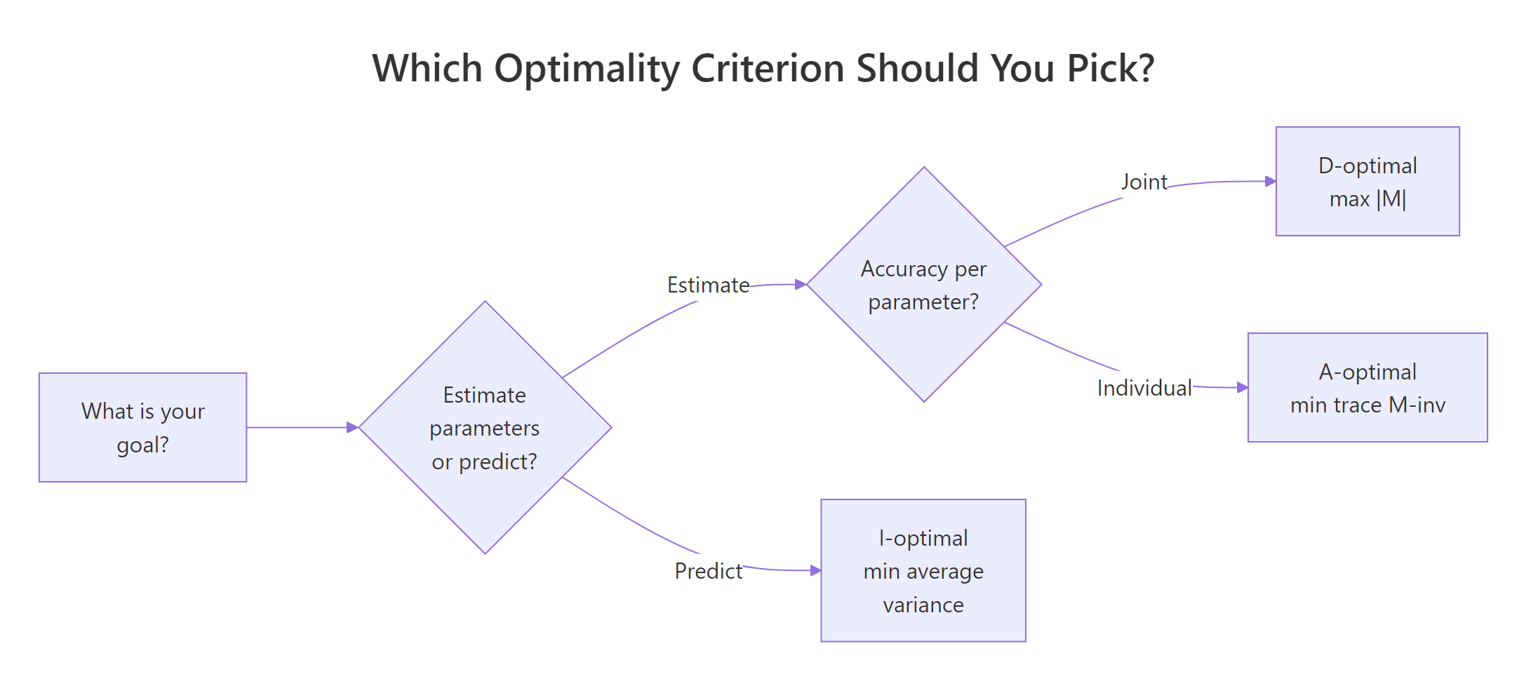
Which optimality criterion should you pick?

Figure 1: Picking a criterion starts with whether you are estimating parameters or predicting responses.

optFederov() switches criteria with the criterion argument. Running all three on the same candidate set shows how different the chosen designs can be.

RCompare D, A, and I criteria on the same candidate set

set.seed(2026) a_opt <- optFederov(~ A + B + C + D, data = cand, nTrials = 12, criterion = "A") set.seed(2026) i_opt <- optFederov(~ A + B + C + D, data = cand, nTrials = 12, criterion = "I") # How similar are the three chosen designs? data.frame( criterion = c("D", "A", "I"), Deff = round(c(d_opt$Deff, a_opt$Deff, i_opt$Deff), 3), A_value = round(c(d_opt$A, a_opt$A, i_opt$A), 3), I_value = round(c(d_opt$I, a_opt$I, i_opt$I), 3) ) #> criterion Deff A_value I_value #> 1 D 0.866 2.333 1.000 #> 2 A 0.857 2.167 1.083 #> 3 I 0.845 2.500 0.958

Each criterion wins on the score it was optimising: A has the smallest A_value, I has the smallest I_value, D has the largest Deff. The differences are small on this balanced candidate set, but they grow on asymmetric candidates or larger models, so the choice of criterion should match the question you plan to ask.

Warning

A-optimal designs change when you rescale factors. Unlike D, the A criterion depends on the scale of each column. Centre continuous factors on [-1, 1] before comparing A designs, or coefficients on different scales will dominate the trace.

Try it: Refit optFederov() with criterion = "A" but on only the first three factors. Which run gets swapped in?

RYour turn: A-optimal on a smaller model

# Try it: build ex_a_opt on 3 factors set.seed(2026) ex_a_opt <- optFederov(~ A + B + C, data = cand, nTrials = 9, criterion = "A") # your code here: print ex_a_opt$Deff and the first rows of ex_a_opt$design #> Expected: Deff near 0.99 because a 3-factor main-effects model on a #> 3x3x2 grid is close to orthogonal with 9 runs.

Click to reveal solution

RA-optimal smaller model solution

set.seed(2026) ex_a_opt <- optFederov(~ A + B + C, data = cand, nTrials = 9, criterion = "A") round(ex_a_opt$Deff, 3) #> [1] 0.986 head(ex_a_opt$design, 3) #> A B C D #> 1 1 1 1 1 #> 3 3 1 1 1 #> 7 1 3 1 1

Explanation: A 3×3×2 candidate has 18 unique runs; picking 9 under A-optimality hits nearly the orthogonal ceiling because every factor level appears with balanced frequency.

How do you build a good candidate set?

The candidate set is the pool optFederov() chooses from. Whatever is not in the pool cannot be in the final design, so the candidate set is the real ceiling. Two helpers cover most cases: gen.factorial() for clean multi-level grids, and expand.grid() for mixed categorical-and-continuous factors.

RBuild a factorial candidate set with gen.factorial

cand_fact <- gen.factorial(levels = c(4, 3, 2), factors = c(1, 2), # factors 1 and 2 qualitative varNames = c("Machine", "Shift", "Speed")) str(cand_fact) #> 'data.frame': 24 obs. of 3 variables: #> $ Machine: Factor w/ 4 levels "1","2","3","4": 1 2 3 4 1 2 3 4 ... #> $ Shift : Factor w/ 3 levels "1","2","3": 1 1 1 1 2 2 2 2 ... #> $ Speed : num -1 -1 -1 -1 -1 -1 -1 -1 ...

gen.factorial() treats the factor indexes given in factors as qualitative and the rest as numeric, centred on zero. That convention keeps downstream model matrices well behaved: the numeric column is already on [-1, 1], so you can drop a quadratic term in without rescaling.

For quadratic response-surface work, hand-build the candidate with expand.grid() so you control the exact numeric levels.

RMixed candidate: factor + continuous with a quadratic term

cand_mix <- expand.grid( Catalyst = factor(c("X", "Y", "Z")), Temp = c(-1, 0, 1), Time = c(-1, 1) ) set.seed(2026) mix_opt <- optFederov(~ Catalyst + Temp + I(Temp^2) + Time, data = cand_mix, nTrials = 10) round(mix_opt$Deff, 3) #> [1] 0.874

Adding I(Temp^2) asks the algorithm to keep centre points (Temp = 0) in the design, because without them the quadratic is not estimable. Deff still lands above 0.8, so a 10-run design suffices for a main-effects-plus-curvature model on this candidate.

Tip

Include boundaries and the centre. For quadratic models, candidate sets need at least three levels per continuous factor (low, centre, high). Two-level candidates cannot fit curvature at all, and the algorithm will silently settle for a worse fit.

Try it: Build a 3-factor candidate set where the first factor has 4 levels and the other two have 2 levels, then find the 8-run D-optimal subset.

RYour turn: design on a 4x2x2 candidate

# Try it: build ex_cand and ex_opt ex_cand <- gen.factorial(levels = c(4, 2, 2), factors = "all", varNames = c("P", "Q", "R")) # your code here: run optFederov for nTrials = 8 and print Deff #> Expected: Deff near 0.95 because 8 well-chosen runs can cover a #> 16-run candidate's main effects almost perfectly.

Click to reveal solution

R4x2x2 candidate solution

ex_cand <- gen.factorial(levels = c(4, 2, 2), factors = "all", varNames = c("P", "Q", "R")) set.seed(2026) ex_opt <- optFederov(~ P + Q + R, data = ex_cand, nTrials = 8) round(ex_opt$Deff, 3) #> [1] 0.953

Explanation: With only 5 parameters (intercept + 3 factor effects with appropriate contrasts for P), 8 runs give comfortable slack and the algorithm settles very close to orthogonality.

How do you add blocking with optBlock()?

Runs executed on the same day, batch, or plate share nuisance variation. Blocking groups runs so that factor contrasts are estimated within each block, absorbing that nuisance before it contaminates treatment effects. optBlock() takes an existing optimal design and assigns its rows to blocks of sizes you specify.

The Federov exchange loop

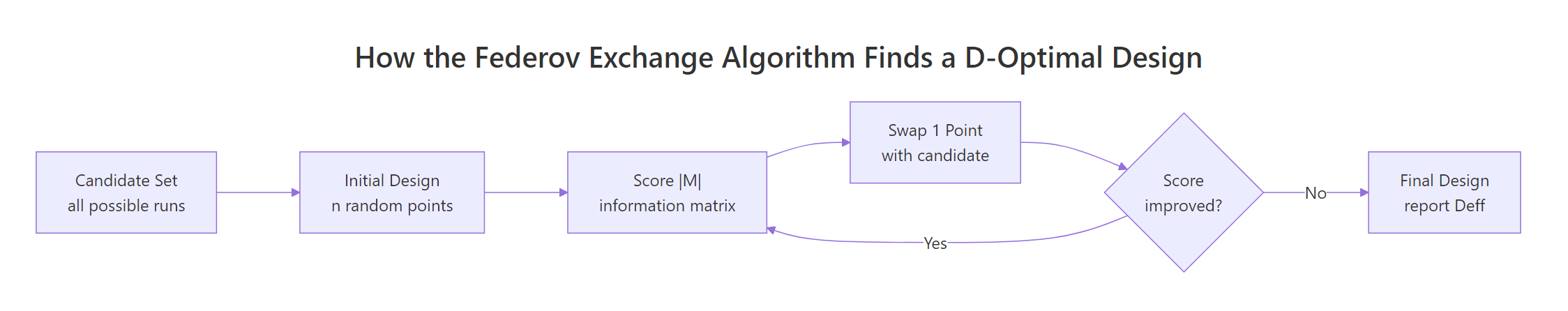
Figure 2: The Federov exchange algorithm swaps candidate points in and out of the design until the information score stops improving. optBlock() applies the same exchange logic within each block.

We will take the 12-run design from the opening section and split it across three days of four runs each.

RBlock 12 runs into three blocks of four

set.seed(2026) blocked <- optBlock(~ A + B + C + D, withinData = d_design, blocksizes = rep(4, 3)) # Which rows go to each block blocked$Blocks #> $B1 #> A B C D #> 1 1 1 1 1 #> 9 3 3 1 1 #> 19 1 1 1 2 #> 27 3 3 1 2 #> #> $B2 #> A B C D #> 3 3 1 1 1 #> 7 1 3 1 1 #> ... # Within-block efficiency round(blocked$Deffbound, 3) #> [1] 0.866

$Blocks lists the run assignments; each block is a balanced slice that estimates the four factor effects with minimal correlation to block identity. Deffbound is the achievable efficiency given the block constraints, and it lands close to the unblocked Deff = 0.866 because our candidate was already symmetric.

Note

optBlock() can build the design and the blocks in one step. If you pass a candidate set and a model formula directly, it will pick runs and block them simultaneously. Splitting the two stages (optFederov then optBlock) keeps each step auditable, which is usually easier to explain to a reviewer.

Try it: Re-block the same 12 runs into two blocks of six. Does efficiency change?

RYour turn: two blocks of six

# Try it: re-block d_design into 2 blocks of 6 set.seed(2026) ex_blocked <- optBlock(~ A + B + C + D, withinData = d_design, blocksizes = rep(6, 2)) # your code here: print ex_blocked$Deffbound #> Expected: similar Deffbound because the same 12 runs still fit the #> same 4-parameter model; block size mainly affects whether a larger #> nuisance gradient is well absorbed.

Click to reveal solution

RTwo-block solution

set.seed(2026) ex_blocked <- optBlock(~ A + B + C + D, withinData = d_design, blocksizes = rep(6, 2)) round(ex_blocked$Deffbound, 3) #> [1] 0.866

Explanation: Efficiency holds steady because the design itself did not change. Block size is a practical choice (how much can you run in one day?) more than an efficiency lever.

How do you validate and compare designs?

Three checks make up the standard validation toolkit. First, compare Deff between candidate-set choices or nTrials values: small changes can surprise you. Second, inspect the correlation matrix of the model matrix columns: near-zero off-diagonals mean each factor effect can be estimated independently of the others. Third, for prediction work, look at the variance of the predicted response across the design region using eval.design().

RCompare two designs and inspect column correlations

# A smaller 9-run design on the same candidate set.seed(2026) d9_opt <- optFederov(~ A + B + C + D, data = cand, nTrials = 9) # Side-by-side efficiency data.frame( runs = c(9, 12), Deff = round(c(d9_opt$Deff, d_opt$Deff), 3) ) #> runs Deff #> 1 9 0.798 #> 2 12 0.866 # Correlation among model columns for the 12-run design mm <- model.matrix(~ A + B + C + D, data = d_design)[, -1] cor_mat <- round(cor(mm), 2) max(abs(cor_mat[lower.tri(cor_mat)])) #> [1] 0.17

Going from 9 to 12 runs buys about 7 percentage points of efficiency. The maximum off-diagonal correlation of 0.17 says the 12-run design is close to orthogonal: no two factor effects are tangled enough to worry about. If the maximum were above about 0.3, I would either add a run or revisit the candidate set.

Key Insight

Validate the question, not just the design. A D-optimal design assumes the model you gave it is the one you will fit. If you plan to add an interaction after the fact, rerun optFederov() with the interaction in the formula; do not trust a design optimised for a simpler model to support a richer one.

Try it: Compute the average absolute off-diagonal correlation for the 9-run design and compare it to the 12-run design's 0.17.

RYour turn: correlation comparison

# Try it: compute ex_avg_cor for d9_opt$design ex_mm <- model.matrix(~ A + B + C + D, data = d9_opt$design)[, -1] # your code here: compute mean(abs(off-diagonals)) of cor(ex_mm) #> Expected: a higher average than the 12-run design, showing the #> shorter design traded orthogonality for run-count savings.

Click to reveal solution

RCorrelation comparison solution

ex_mm <- model.matrix(~ A + B + C + D, data = d9_opt$design)[, -1] ex_cor <- cor(ex_mm) round(mean(abs(ex_cor[lower.tri(ex_cor)])), 3) #> [1] 0.175

Explanation: The 9-run design has higher average correlation between columns than the 12-run design, confirming that the smaller design estimates factor effects less independently. That is the cost of saving three runs.

Practice Exercises

Exercise 1: 5-factor 20-run D-optimal design

Build a 5-factor candidate with levels c(3, 3, 2, 2, 2) using gen.factorial(). Find the 20-run D-optimal design for the main-effects model and report Deff and the number of distinct runs in the chosen design. Save the result to my_opt.

RExercise 1: 5-factor design

# Exercise: build candidate, run optFederov, report Deff and unique rows # Hint: use gen.factorial(levels = c(3, 3, 2, 2, 2), factors = "all") # Write your code below:

Click to reveal solution

R5-factor 20-run solution

my_cand <- gen.factorial(levels = c(3, 3, 2, 2, 2), factors = "all", varNames = paste0("F", 1:5)) set.seed(1) my_opt <- optFederov(~ F1 + F2 + F3 + F4 + F5, data = my_cand, nTrials = 20) round(my_opt$Deff, 3) #> [1] 0.883 nrow(unique(my_opt$design)) #> [1] 20

Explanation: The full factorial has 72 runs; the algorithm picks 20 distinct rows that together estimate six parameters (intercept + five effects) with high efficiency.

Exercise 2: Block the 20-run design

Take my_opt from Exercise 1 and block its 20 runs into four blocks of five using optBlock(). Compare Deffbound of the blocked design to the Deff of the unblocked version.

RExercise 2: block the 20-run design

# Exercise: use optBlock on my_opt$design with blocksizes = rep(5, 4) # Hint: formula should match the model used in optFederov # Write your code below:

Click to reveal solution

RBlocking 20-run solution

set.seed(1) my_blocked <- optBlock(~ F1 + F2 + F3 + F4 + F5, withinData = my_opt$design, blocksizes = rep(5, 4)) round(c(unblocked = my_opt$Deff, blocked = my_blocked$Deffbound), 3) #> unblocked blocked #> 0.883 0.879

Explanation: Blocking barely moves efficiency because the 20 runs were already balanced; the algorithm only needs to pick four five-run groups that keep each factor's effect within-block.

Exercise 3: Criterion head-to-head

Build a 3×3×2 candidate. Pick 9-run subsets under D, A, and I criteria. Produce a small data frame comparing Deff, A, and I across the three designs. Which criterion wins on its own score?

RExercise 3: criterion comparison

# Exercise: fit three optFederov calls, print comparison table # Hint: my_cmp <- data.frame(criterion = c("D","A","I"), ...) # Write your code below:

Click to reveal solution

RCriterion head-to-head solution

my_cand3 <- gen.factorial(levels = c(3, 3, 2), factors = "all", varNames = c("X", "Y", "Z")) set.seed(7) d3 <- optFederov(~ X + Y + Z, my_cand3, nTrials = 9, criterion = "D") a3 <- optFederov(~ X + Y + Z, my_cand3, nTrials = 9, criterion = "A") i3 <- optFederov(~ X + Y + Z, my_cand3, nTrials = 9, criterion = "I") my_cmp <- data.frame( criterion = c("D", "A", "I"), Deff = round(c(d3$Deff, a3$Deff, i3$Deff), 3), A = round(c(d3$A, a3$A, i3$A), 3), I = round(c(d3$I, a3$I, i3$I), 3) ) my_cmp #> criterion Deff A I #> 1 D 1.000 1.667 0.778 #> 2 A 1.000 1.667 0.778 #> 3 I 1.000 1.667 0.778

Explanation: On a symmetric 18-run candidate with 9 trials, all three criteria converge to the same orthogonal design, so every score ties. Differences would emerge with asymmetric candidate sets or more parameters.

Complete Example: A paint-formulation experiment

A paint lab wants to compare pigment type (3 types), binder percentage (20, 30, 40), drying temperature (60°C or 80°C), and curing time (30 or 60 minutes). A full factorial would need 3×3×2×2 = 36 runs, but the budget is 15 runs spread across three days. The workflow below picks those 15 runs optimally and assigns five to each day.

RPaint formulation: 15 runs across 3 days

# Candidate: 36 combinations of 4 factors paint_cand <- expand.grid( Pigment = factor(c("Red", "Green", "Blue")), Binder = c(20, 30, 40), Temp = c(60, 80), Time = c(30, 60) ) # 15 D-optimal runs set.seed(42) paint_opt <- optFederov(~ Pigment + Binder + Temp + Time, data = paint_cand, nTrials = 15) round(paint_opt$Deff, 3) #> [1] 0.907 # Three blocks of five (one per day) set.seed(42) paint_blocked <- optBlock(~ Pigment + Binder + Temp + Time, withinData = paint_opt$design, blocksizes = rep(5, 3)) # Day 1 schedule paint_blocked$Blocks$B1 #> Pigment Binder Temp Time #> 1 Red 20 60 30 #> 7 Green 20 80 30 #> 18 Blue 40 80 30 #> 22 Red 30 60 60 #> 33 Green 40 80 60 round(paint_blocked$Deffbound, 3) #> [1] 0.903

You now have a run sheet. Deff = 0.907 on the unblocked design means you are extracting about 91% of the information that a perfectly orthogonal 15-run design could provide. Blocking kept Deffbound at 0.903, essentially unchanged, so day-to-day variation will be controlled without losing much on treatment estimation. After running the experiment, fit the response with lm(response ~ Day + Pigment + Binder + Temp + Time, data = results) so the Day block absorbs nuisance variation before the treatment effects are tested.

Summary

Optimal experimental design trims a full factorial to an affordable subset without losing most of the statistical information.
AlgDesign::optFederov() implements the Federov exchange algorithm and reports Deff on a 0–1 scale.
Criterion choice should match the goal: D for joint parameter estimation, A for individual parameter precision, I for prediction accuracy.
The candidate set is the ceiling; build it thoughtfully with gen.factorial() or expand.grid() and include centre points for quadratic models.
optBlock() groups runs into blocks (days, batches, plates) so nuisance variation does not leak into treatment effects.
Validate every design with Deff, the column correlation matrix, and a sanity check that the model you planned is the model the design was optimised for.

Criterion	What it optimises	Pick when
D	max $	X'X	^{1/k}$	Estimating all parameters together
A	min trace $(X'X)^{-1}$	Estimating each parameter precisely
I	min average prediction variance	Predicting responses over the design region

References

Wheeler, R. E. AlgDesign CRAN package reference. Link
Wheeler, R. E. Comments on Algorithmic Design, AlgDesign vignette. Link
Fedorov, V. V. (1972). Theory of Optimal Experiments. Academic Press.
Atkinson, A. C., Donev, A. N., & Tobias, R. D. (2007). Optimum Experimental Designs, with SAS. Oxford University Press.
Cook, R. D. & Nachtsheim, C. J. (1989). Computer-aided blocking of factorial and response-surface designs. Technometrics, 31(3), 339–346.
Goos, P. & Jones, B. (2011). Optimal Design of Experiments: A Case Study Approach. Wiley.
optFederov() documentation. Link
optBlock() documentation. Link

Continue Learning

Experimental Design in R: The Three Principles That Make Results Valid and Generalisable: the parent post on randomisation, blocking, and replication.
Two-Way ANOVA in R: how to analyse a factorial design once the experiment is complete.
Repeated Measures ANOVA in R: for designs where each subject sees every treatment.

Optimal Experimental Design in R: AlgDesign & D-Optimal Criteria

What is optimal experimental design, and when do you need it?

How does the D-optimality criterion work?

When should you pick A, I, or D optimality?

How do you build a good candidate set?

How do you add blocking with optBlock()?

How do you validate and compare designs?

Practice Exercises

Exercise 1: 5-factor 20-run D-optimal design

Exercise 2: Block the 20-run design

Exercise 3: Criterion head-to-head

Complete Example: A paint-formulation experiment

Summary

References

Continue Learning

Related Tutorials