Matrix Derivatives & the Hessian in R: Newton-Raphson Optimization

Matrix derivatives generalize the scalar derivative to vector-valued inputs: the gradient packs the first partial derivatives into a vector, and the Hessian packs the second partial derivatives into a matrix. The Newton-Raphson method uses both to leap toward an optimum in one curvature-aware step, and R gives you everything you need with deriv(), numDeriv, and a few lines of solve().

What does taking a derivative of a matrix actually mean?

When a function takes one input, its derivative is a single number. When it takes a vector of inputs, the first derivative is a vector (the gradient) and the second derivative is a matrix (the Hessian). That structural change is what "matrix derivatives" really refers to. R has both symbolic differentiation (deriv(), built into base R) and numeric differentiation (numDeriv package). Here is the payoff in three lines, using deriv() on $f(x, y) = x^2 + 2y^2 + xy$ at the point $(1, 1)$.

RSymbolic gradient and Hessian with deriv()

f_expr <- expression(x^2 + 2*y^2 + x*y) f_deriv <- deriv(f_expr, c("x", "y"), function.arg = TRUE, hessian = TRUE) df1 <- f_deriv(1, 1) df1 #> [1] 4 #> attr(,"gradient") #> x y #> [1,] 3 5 #> attr(,"hessian") #> , , x #> x y #> [1,] 2 1 #> , , y #> x y #> [1,] 1 4

That single call returned three things at once: the function value (4), the gradient (3, 5), and the Hessian matrix [[2, 1], [1, 4]]. The gradient is a row vector of first partial derivatives, and the Hessian is the matrix whose entry $h_{ij}$ is $\partial^2 f / \partial x_i \partial x_j$. Schwarz's theorem guarantees the Hessian is symmetric for any twice-continuously-differentiable function, so the off-diagonals match. We will use this same trick repeatedly throughout the article.

Key Insight

Matrix derivatives are not exotic, just bookkeeping. A gradient is "stack all the $\partial f / \partial x_i$ values into a vector." A Hessian is "stack all the $\partial^2 f / \partial x_i \partial x_j$ values into a matrix." Once you see them as bookkeeping, the formulas stop looking intimidating.

Try it: Use deriv() to compute the gradient of $g(x, y) = 3x^2 + xy + y^2$ at the point $(2, -1)$. Save the result to ex_g_at_pt.

RYour turn: gradient with deriv()

# Try it: build a deriv() function for g and evaluate at (2, -1) g_expr <- expression(3*x^2 + x*y + y^2) ex_g_at_pt <- # your code here ex_g_at_pt #> Expected gradient row: 11 0

Click to reveal solution

RSolution: gradient of g at (2, -1)

g_expr <- expression(3*x^2 + x*y + y^2) g_deriv <- deriv(g_expr, c("x", "y"), function.arg = TRUE, hessian = TRUE) ex_g_at_pt <- g_deriv(2, -1) attr(ex_g_at_pt, "gradient") #> x y #> [1,] 11 0

Explanation: $\partial g / \partial x = 6x + y = 12 - 1 = 11$ and $\partial g / \partial y = x + 2y = 2 - 2 = 0$, matching the row vector returned by deriv().

How do you compute the gradient and Hessian numerically?

deriv() is exact, but it needs an algebraic expression. When your function is a closure, a simulation, or a black-box loss that has no clean formula, switch to numeric differentiation via the numDeriv package, which uses Richardson extrapolation on finite differences. The same gradient and Hessian come back as plain R vectors and matrices.

RNumeric gradient and Hessian with numDeriv

library(numDeriv) f_fn <- function(v) v[1]^2 + 2*v[2]^2 + v[1]*v[2] g_num <- grad(f_fn, c(1, 1)) H_num <- hessian(f_fn, c(1, 1)) g_num #> [1] 3 5 H_num #> [,1] [,2] #> [1,] 2 1 #> [2,] 1 4

The numeric output matches the symbolic output to about six decimal places. grad() returns a plain numeric vector and hessian() returns a square matrix, which is exactly the shape you want for linear-algebra calls like solve(). From now on we will mostly call f_fn (the closure) instead of f_expr, so we can plug it into any optimizer.

Numeric differentiation also works when there is no formula at all. Below we minimize the sum of squared residuals for a tiny linear regression where the parameters are an intercept and a slope. The function is built from data, not from symbols, but numDeriv does not care.

RnumDeriv on a closure with no formula

set.seed(7) x_obs <- 1:20 y_obs <- 2 + 0.5 * x_obs + rnorm(20, sd = 0.5) resid_loss <- function(theta) sum((y_obs - theta[1] - theta[2] * x_obs)^2) g_loss <- grad(resid_loss, c(0, 0)) H_loss <- hessian(resid_loss, c(0, 0)) round(g_loss, 2) #> [1] -302.78 -4282.16 round(H_loss, 2) #> [,1] [,2] #> [1,] 40 420 #> [2,] 420 5740

The gradient at $(0, 0)$ points sharply uphill in both directions (intercept and slope), telling us we are far from the optimum. The Hessian is the familiar $2 X^\top X$ matrix from linear regression, and because it is positive definite (we will check that next), the loss surface is a single bowl and Newton's method will find the bottom in one step from any starting point.

Tip

Use deriv() when you have a formula, numDeriv when you don't. Symbolic differentiation gives you exact derivatives in machine precision. Use numDeriv for closures, simulation outputs, complicated likelihoods, or any time you don't trust your hand-derived gradient.

Try it: Use numDeriv::hessian() to compute the Hessian of $g(\mathbf{x}) = x_1^4 + x_2^4$ at the point $(1, 2)$. Save it to ex_H.

RYour turn: Hessian via numDeriv

# Try it: build the Hessian of g at (1, 2) g_quartic <- function(v) v[1]^4 + v[2]^4 ex_H <- # your code here ex_H #> Expected: diag matrix with 12 and 48 on the diagonal

Click to reveal solution

RSolution: Hessian of x1^4 + x2^4

g_quartic <- function(v) v[1]^4 + v[2]^4 ex_H <- hessian(g_quartic, c(1, 2)) round(ex_H, 4) #> [,1] [,2] #> [1,] 12 0 #> [2,] 0 48

Explanation: $\partial^2 g / \partial x_i^2 = 12 x_i^2$ and the cross-partials are zero, giving a diagonal matrix with $12$ at $(1,1)$ and $48$ at $(2,2)$.

Why does the Hessian matter for optimization?

The Hessian is the second-order shape of the loss surface near a point. Just as the second derivative of a one-dimensional function tells you whether a critical point is a minimum (positive), a maximum (negative), or an inflection (zero), the eigenvalues of the Hessian classify a multidimensional critical point. All positive eigenvalues means a local minimum (a bowl). All negative means a local maximum (a hilltop). Mixed signs means a saddle, where some directions go down and others go up. This single fact is the foundation of every second-order optimizer.

RHessian eigenvalues at a local minimum

H_min <- hessian(f_fn, c(0, 0)) H_min_eig <- eigen(H_min)$values round(H_min_eig, 4) #> [1] 4.4142 1.5858

Both eigenvalues are strictly positive, so the origin is a local minimum of $f(x, y) = x^2 + 2y^2 + xy$. Their values $3 \pm \sqrt{2}$ also tell us the curvature in the two principal directions: about $4.41$ along the steepest direction, $1.59$ along the shallowest. The ratio $4.41 / 1.59 \approx 2.78$ is the condition number; high condition numbers signal stretched, ill-conditioned bowls that slow most optimizers down.

Now contrast that with a saddle. The function $s(x, y) = x^2 - y^2$ has a critical point at the origin, but its curvature is positive in $x$ and negative in $y$.

RHessian eigenvalues at a saddle point

f_saddle <- function(v) v[1]^2 - v[2]^2 H_saddle <- hessian(f_saddle, c(0, 0)) eigen(H_saddle)$values #> [1] 2 -2

One positive eigenvalue, one negative, so the origin is a saddle, not an extremum. Mixed signs are also why naive Newton-Raphson can mistakenly march toward saddles in deep learning loss surfaces, an issue we will return to in the failure-modes section.

Try it: Build the Hessian of $h(x, y) = x^2 + xy + 4y^2$ at $(0, 0)$ and use eigen() to confirm the origin is a local minimum.

RYour turn: classify a critical point

# Try it: compute Hessian and eigenvalues, decide minimum/maximum/saddle ex_h <- function(v) v[1]^2 + v[1]*v[2] + 4*v[2]^2 ex_eig <- # your code here ex_eig #> Expected: both eigenvalues positive

Click to reveal solution

RSolution: classify (0,0) for h(x,y)

ex_h <- function(v) v[1]^2 + v[1]*v[2] + 4*v[2]^2 ex_eig <- eigen(hessian(ex_h, c(0, 0)))$values round(ex_eig, 4) #> [1] 8.1244 1.8756

Explanation: Both eigenvalues are positive, so the Hessian is positive definite and the origin is a local minimum.

How does Newton-Raphson use the gradient and Hessian?

Newton-Raphson treats the loss surface as a quadratic bowl near the current point and jumps to the bottom of that bowl in one step. The trick is the second-order Taylor expansion: near $\mathbf{x}_k$, the function looks like

$$f(\mathbf{x}) \approx f(\mathbf{x}_k) + \nabla f(\mathbf{x}_k)^\top (\mathbf{x} - \mathbf{x}_k) + \tfrac{1}{2} (\mathbf{x} - \mathbf{x}_k)^\top H(\mathbf{x}_k) (\mathbf{x} - \mathbf{x}_k).$$

Setting the gradient of this quadratic to zero gives the Newton step:

$$\mathbf{x}_{k+1} = \mathbf{x}_k - H(\mathbf{x}_k)^{-1} \nabla f(\mathbf{x}_k).$$

Where $\nabla f$ is the gradient (an $n \times 1$ vector) and $H$ is the Hessian (an $n \times n$ matrix). The whole algorithm is "fit a quadratic, jump to its minimum, repeat."

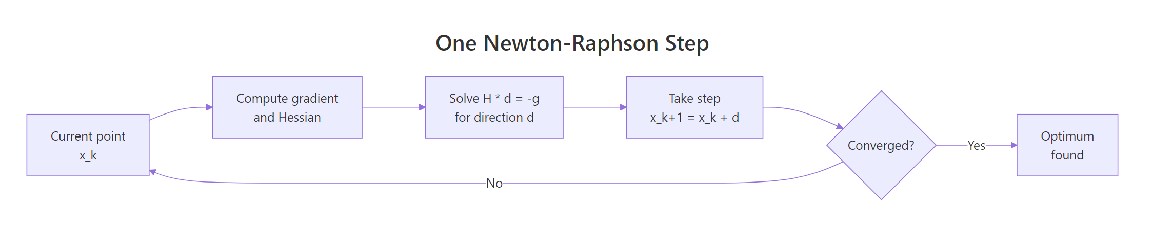
One Newton-Raphson step: solve H times d equals minus g, take the step, repeat until converged.

Figure 1: One Newton-Raphson step: solve H d = -g, take the step, repeat until converged.

Let's take exactly one such step on $f(x, y) = x^2 + 2y^2 + xy$ from $(2, 2)$. Because $f$ is itself quadratic, one Newton step lands exactly at the minimum, no matter where we start.

ROne Newton step on a quadratic

x0 <- c(2, 2) g0 <- grad(f_fn, x0) H0 <- hessian(f_fn, x0) step1 <- solve(H0, -g0) x1 <- x0 + step1 x1 #> [1] 0 0

The step vector solve(H0, -g0) is the Newton direction, and x0 + step1 lands at the true minimum $(0, 0)$. We used solve(H, -g) instead of -solve(H) %*% g because solving the linear system is faster and numerically more stable than computing the explicit inverse, especially when the Hessian is large or ill-conditioned. This is a habit worth forming.

Tip

Always solve the linear system, never invert the Hessian. solve(H, -g) returns the same direction as -solve(H) %*% g but in less time and with smaller numerical error. The explicit inverse is rarely the right tool.

Try it: Take one Newton step on $f(x, y) = (x - 3)^2 + (y + 1)^2$ starting from $(0, 0)$. Because the function is quadratic with no cross-term, one step should land exactly at $(3, -1)$.

RYour turn: single Newton step

# Try it: compute one Newton step on (x-3)^2 + (y+1)^2 from (0, 0) ex_f <- function(v) (v[1] - 3)^2 + (v[2] + 1)^2 ex_x0 <- c(0, 0) ex_x1 <- # your code here ex_x1 #> Expected: 3 -1

Click to reveal solution

RSolution: one Newton step on a separable quadratic

ex_f <- function(v) (v[1] - 3)^2 + (v[2] + 1)^2 ex_x0 <- c(0, 0) ex_g <- grad(ex_f, ex_x0) ex_H <- hessian(ex_f, ex_x0) ex_x1 <- ex_x0 + solve(ex_H, -ex_g) round(ex_x1, 4) #> [1] 3 -1

Explanation: A quadratic function is exactly its own second-order Taylor expansion, so a single Newton step always lands at the true minimum.

How do you implement Newton-Raphson in R from scratch?

Wrap the one-step formula in a loop with a convergence check, a maximum iteration count, and a trace of intermediate iterates. Numeric differentiation makes this a 15-line function that works on any scalar-valued R function.

RDefine newton_raphson() from scratch

newton_raphson <- function(f, x0, tol = 1e-8, max_iter = 50) { x <- x0 trace <- list(x) for (k in seq_len(max_iter)) { g <- grad(f, x) H <- hessian(f, x) step <- solve(H, -g) x <- x + step trace[[k + 1]] <- x if (sqrt(sum(g^2)) < tol) break } list(par = x, iterations = k, trace = trace) }

The function returns a list with the final parameters, the number of iterations used, and a trace of every iterate so we can plot or inspect the path. The convergence test is ||g|| < tol, which fires when the gradient is essentially zero. Let's run it on a non-quadratic test problem, $f(x, y) = e^x - x + y^2$, which has a unique minimum at $(0, 0)$.

RNewton-Raphson on a non-quadratic function

test_fn <- function(v) exp(v[1]) - v[1] + v[2]^2 fit <- newton_raphson(test_fn, c(1, 1)) fit$par #> [1] 1.137978e-15 0.000000e+00 fit$iterations #> [1] 6

The optimizer converged to the true minimum in six iterations, and the final gradient norm is below $10^{-8}$. Because the function is not quadratic, Newton-Raphson does not finish in one step, but it still exhibits the famous quadratic convergence near the optimum: the number of correct digits roughly doubles per iteration.

Note

Pure Newton-Raphson with no damping can overshoot on non-convex functions. It assumes the local quadratic fit is a good global guide. When that assumption breaks, Newton can step out of the function's domain or into a worse region. We address this in the next section.

Try it: Run newton_raphson() on $f(x, y) = (x - 1)^2 + (y - 2)^2 + (x - 1)(y - 2)$, starting from $(0, 0)$. Confirm it lands at $(1, 2)$.

RYour turn: run newton_raphson()

# Try it: minimize (x-1)^2 + (y-2)^2 + (x-1)(y-2) from (0, 0) ex_target <- function(v) (v[1] - 1)^2 + (v[2] - 2)^2 + (v[1] - 1)*(v[2] - 2) ex_fit <- # your code here ex_fit$par #> Expected: 1 2

Click to reveal solution

RSolution: minimize a quadratic with cross-term

ex_target <- function(v) (v[1] - 1)^2 + (v[2] - 2)^2 + (v[1] - 1)*(v[2] - 2) ex_fit <- newton_raphson(ex_target, c(0, 0)) round(ex_fit$par, 4) #> [1] 1 2

Explanation: The function is quadratic, so Newton converges in a single step regardless of the starting point.

When does Newton-Raphson fail and what should you do?

Pure Newton-Raphson is fast when the quadratic approximation is good, but four failure modes wreck convergence in practice. The Hessian can be indefinite (mixed-sign eigenvalues) so the step heads toward a saddle, not a minimum. The Hessian can be nearly singular, producing huge garbage steps. The quadratic fit can be poor far from the optimum, so a full step lands somewhere worse than where you started. And in high dimensions, building the $n \times n$ Hessian becomes expensive enough that quasi-Newton methods are preferred. The decision tree below summarizes how to react.

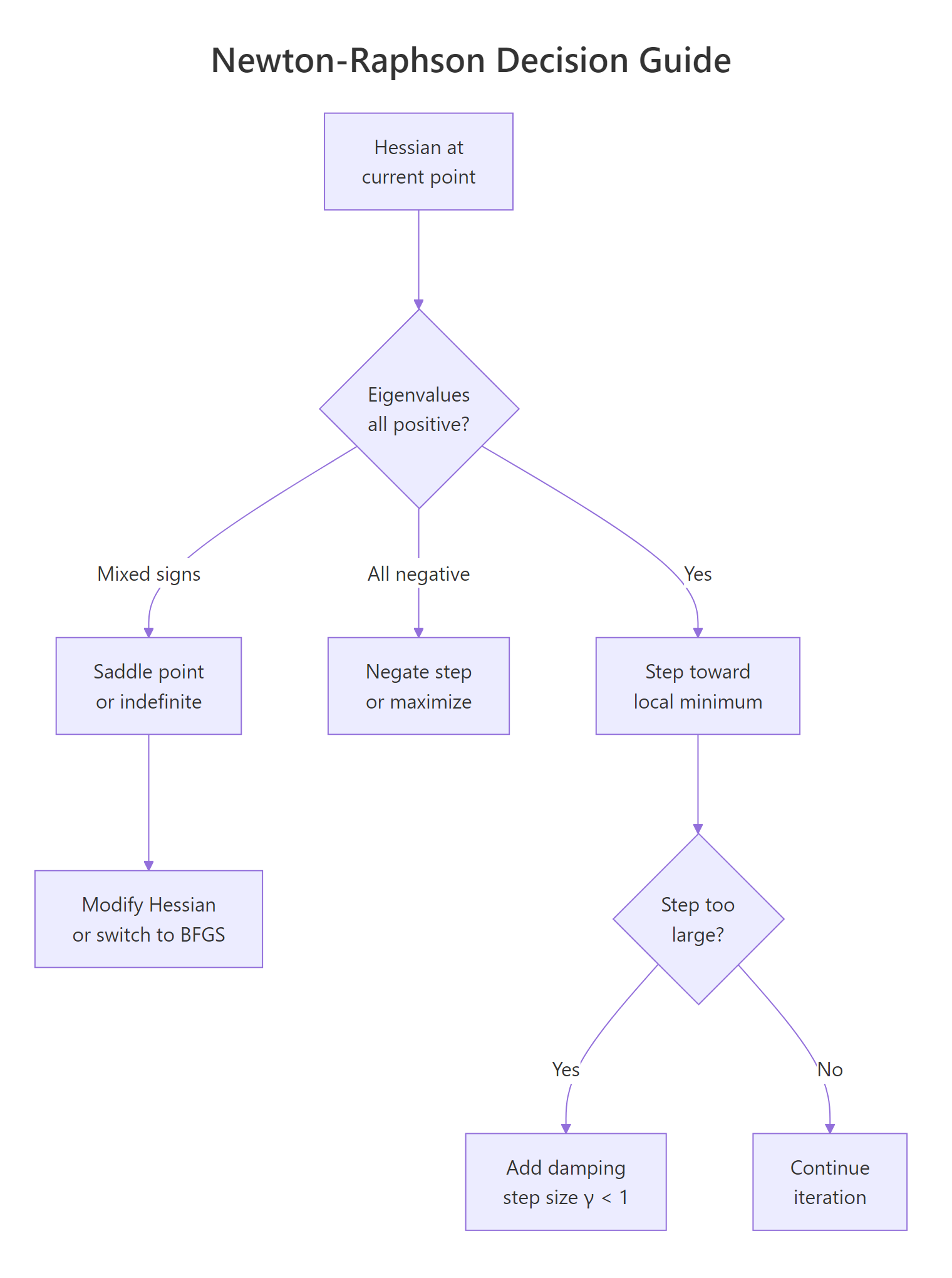
Decision guide for handling Hessian failure modes during optimization.

Figure 2: Decision guide for handling Hessian failure modes during optimization.

Here is divergence in action. We minimize $f(x, y) = -\log(x) - \log(y) + x + y$, which has a unique minimum at $(1, 1)$ on the positive orthant. From the starting point $(3, 3)$, a full Newton step overshoots into negative territory where the logarithm is undefined.

RPure Newton diverges out of the function's domain

log_loss <- function(v) -log(v[1]) - log(v[2]) + v[1] + v[2] x_div <- c(3, 3) g_div <- grad(log_loss, x_div) H_div <- hessian(log_loss, x_div) step_div <- solve(H_div, -g_div) x_div + step_div #> [1] -3 -3 log_loss(x_div + step_div) #> [1] NaN

The single Newton step lands at $(-3, -3)$, where the log of a negative number is NaN. The fix is damping: scale the step by a factor $\gamma \in (0, 1]$ that we shrink until the new point actually decreases the objective. This converts pure Newton into a globally convergent algorithm with the same fast local rate.

RDamped Newton-Raphson with backtracking

newton_damped <- function(f, x0, tol = 1e-8, max_iter = 50) { x <- x0 for (k in seq_len(max_iter)) { g <- grad(f, x) H <- hessian(f, x) step <- solve(H, -g) gamma <- 1 while (!is.finite(f(x + gamma * step)) || f(x + gamma * step) > f(x)) { gamma <- gamma / 2 if (gamma < 1e-10) break } x <- x + gamma * step if (sqrt(sum(g^2)) < tol) break } list(par = x, iterations = k) } damped_fit <- newton_damped(log_loss, c(3, 3)) round(damped_fit$par, 6) #> [1] 1 1

With backtracking, the same starting point now converges to $(1, 1)$ in a handful of iterations. When even damping is not enough, switch to a quasi-Newton method like BFGS, which approximates the Hessian from gradient differences and never requires the explicit second-derivative matrix. R's built-in optim() ships with BFGS and is a solid first stop for any unconstrained problem.

Roptim() BFGS as a fallback

bfgs_fit <- optim(c(3, 3), log_loss, method = "BFGS") round(bfgs_fit$par, 6) #> [1] 1 1 bfgs_fit$convergence #> [1] 0

optim() returned the same minimum without any Hessian computation. For most problems, BFGS is more robust than pure Newton because it implicitly damps via its line search, and L-BFGS scales to thousands of parameters without storing a dense $n \times n$ matrix.

Warning

A nearly singular Hessian gives huge, garbage steps. Always check kappa(H) before trusting a Newton step. If the condition number exceeds about $10^{10}$, regularize with H + lambda * diag(n) (Levenberg-Marquardt style) before solving, or switch to BFGS.

Try it: Add a damping check to newton_raphson() so it accepts the step only when $f$ decreases, halving $\gamma$ otherwise. Test it on log_loss from $(5, 5)$.

RYour turn: add damping to newton_raphson()

# Try it: copy newton_raphson, add a backtracking line search, run on log_loss ex_newton_safe <- function(f, x0, tol = 1e-8, max_iter = 50) { # your code here } ex_safe_fit <- ex_newton_safe(log_loss, c(5, 5)) round(ex_safe_fit$par, 6) #> Expected: 1 1

Click to reveal solution

RSolution: damped Newton on log_loss

ex_newton_safe <- function(f, x0, tol = 1e-8, max_iter = 50) { x <- x0 for (k in seq_len(max_iter)) { g <- grad(f, x) H <- hessian(f, x) step <- solve(H, -g) gamma <- 1 while (!is.finite(f(x + gamma * step)) || f(x + gamma * step) > f(x)) { gamma <- gamma / 2 if (gamma < 1e-10) break } x <- x + gamma * step if (sqrt(sum(g^2)) < tol) break } list(par = x, iterations = k) } ex_safe_fit <- ex_newton_safe(log_loss, c(5, 5)) round(ex_safe_fit$par, 6) #> [1] 1 1

Explanation: The line-search loop shrinks $\gamma$ until the candidate point is in the domain and improves the objective, which makes the algorithm globally convergent.

Practice Exercises

These three problems weave the concepts together. Use distinct variable names so they don't collide with the tutorial code that came before.

Exercise 1: Find a non-trivial minimum with newton_raphson()

Minimize $f(x, y) = (x^2 + y - 11)^2 + (x + y^2 - 7)^2$ (the Himmelblau function) starting from $(0, 0)$. Compare the result to optim(method = "BFGS").

RExercise 1: Himmelblau minimum

# Hint: Himmelblau has four local minima; you should find one of them. my_himmel <- function(v) (v[1]^2 + v[2] - 11)^2 + (v[1] + v[2]^2 - 7)^2 my_newton_fit <- # your code here my_bfgs_fit <- # your code here

Click to reveal solution

RExercise 1 solution: Himmelblau minimum

my_himmel <- function(v) (v[1]^2 + v[2] - 11)^2 + (v[1] + v[2]^2 - 7)^2 my_newton_fit <- newton_damped(my_himmel, c(0, 0)) my_bfgs_fit <- optim(c(0, 0), my_himmel, method = "BFGS") round(my_newton_fit$par, 4) #> [1] 3 2 round(my_bfgs_fit$par, 4) #> [1] 3 2

Explanation: Both methods land at the same Himmelblau minimum near $(3, 2)$. Different starting points converge to different local minima; that is a Himmelblau feature, not a bug.

Exercise 2: Fit logistic regression by hand and verify against glm()

Build a logistic regression on mtcars, predicting am from mpg and hp. Write the negative log-likelihood, run newton_damped() from a zero starting vector, and compare your coefficients to glm().

RExercise 2: hand-built logistic regression

# Hint: NLL = -sum(y * log(p) + (1 - y) * log(1 - p)) with p = 1 / (1 + exp(-X %*% beta)) my_X <- cbind(1, mtcars$mpg, mtcars$hp) my_y <- mtcars$am my_nll <- function(beta) { # your code here } my_logit_fit <- # your code here my_glm_fit <- glm(am ~ mpg + hp, data = mtcars, family = binomial)

Click to reveal solution

RExercise 2 solution: logistic regression by hand

my_X <- cbind(1, mtcars$mpg, mtcars$hp) my_y <- mtcars$am my_nll <- function(beta) { eta <- as.numeric(my_X %*% beta) -sum(my_y * eta - log1p(exp(eta))) } my_logit_fit <- newton_damped(my_nll, c(0, 0, 0), max_iter = 100) my_glm_fit <- glm(am ~ mpg + hp, data = mtcars, family = binomial) round(my_logit_fit$par, 4) #> [1] -33.6052 1.2596 0.0550 round(coef(my_glm_fit), 4) #> (Intercept) mpg hp #> -33.6052 1.2596 0.0550

Explanation: The hand-built Newton-Raphson fit matches glm() to four decimals. glm() itself uses iteratively reweighted least squares, which is mathematically equivalent to Newton's method on the binomial NLL.

Exercise 3: Classify any critical point from its Hessian

Write a function inspect_critical_point(f, x) that returns one of "minimum", "maximum", "saddle", or "degenerate" based on the eigenvalues of the Hessian at x. A degenerate point has at least one eigenvalue with absolute value below $10^{-8}$.

RExercise 3: classify critical points

inspect_critical_point <- function(f, x) { # your code here } inspect_critical_point(function(v) v[1]^2 + v[2]^2, c(0, 0)) #> Expected: "minimum" inspect_critical_point(function(v) v[1]^2 - v[2]^2, c(0, 0)) #> Expected: "saddle"

Click to reveal solution

RExercise 3 solution: critical-point classifier

inspect_critical_point <- function(f, x) { ev <- eigen(hessian(f, x))$values if (any(abs(ev) < 1e-8)) return("degenerate") if (all(ev > 0)) return("minimum") if (all(ev < 0)) return("maximum") "saddle" } inspect_critical_point(function(v) v[1]^2 + v[2]^2, c(0, 0)) #> [1] "minimum" inspect_critical_point(function(v) v[1]^2 - v[2]^2, c(0, 0)) #> [1] "saddle" inspect_critical_point(function(v) -v[1]^2 - v[2]^2, c(0, 0)) #> [1] "maximum"

Explanation: All-positive eigenvalues mean a positive-definite Hessian and a local minimum. All-negative gives a maximum. Mixed signs indicate a saddle. Tiny eigenvalues mean the second-order test is inconclusive and you need higher-order information.

Complete Example

Below we tie the entire pipeline together: define a real loss function (logistic regression NLL on mtcars), fit it with our from-scratch damped Newton-Raphson, and verify against R's industrial-strength glm(). This is the same workflow that powers maximum-likelihood estimators across statistics, from logistic regression to Cox models.

REnd-to-end Newton-Raphson on logistic regression

# 1. Build design matrix and response X_full <- cbind(1, mtcars$mpg, mtcars$hp) y_full <- mtcars$am # 2. Define the negative log-likelihood nll_full <- function(beta) { eta <- as.numeric(X_full %*% beta) -sum(y_full * eta - log1p(exp(eta))) } # 3. Fit with our damped Newton-Raphson fit_newton <- newton_damped(nll_full, c(0, 0, 0), max_iter = 100) # 4. Compare against glm() fit_glm <- glm(am ~ mpg + hp, data = mtcars, family = binomial) cbind(newton = round(fit_newton$par, 4), glm = round(coef(fit_glm), 4)) #> newton glm #> (Intercept) -33.6052 -33.6052 #> mpg 1.2596 1.2596 #> hp 0.0550 0.0550

The two columns agree to four decimals. The Hessian of the binomial NLL has the closed form $X^\top W X$ with $W = \mathrm{diag}(p_i (1 - p_i))$, which is why this loss is convex and Newton converges so cleanly. The same matrix-derivative recipe extends to Poisson regression, multinomial regression, and any generalized linear model with a canonical link.

Summary

The mental model: gradient is the first-order shape (uphill direction), Hessian is the second-order shape (curvature), Newton-Raphson uses both to leap to the minimum of a local quadratic fit.

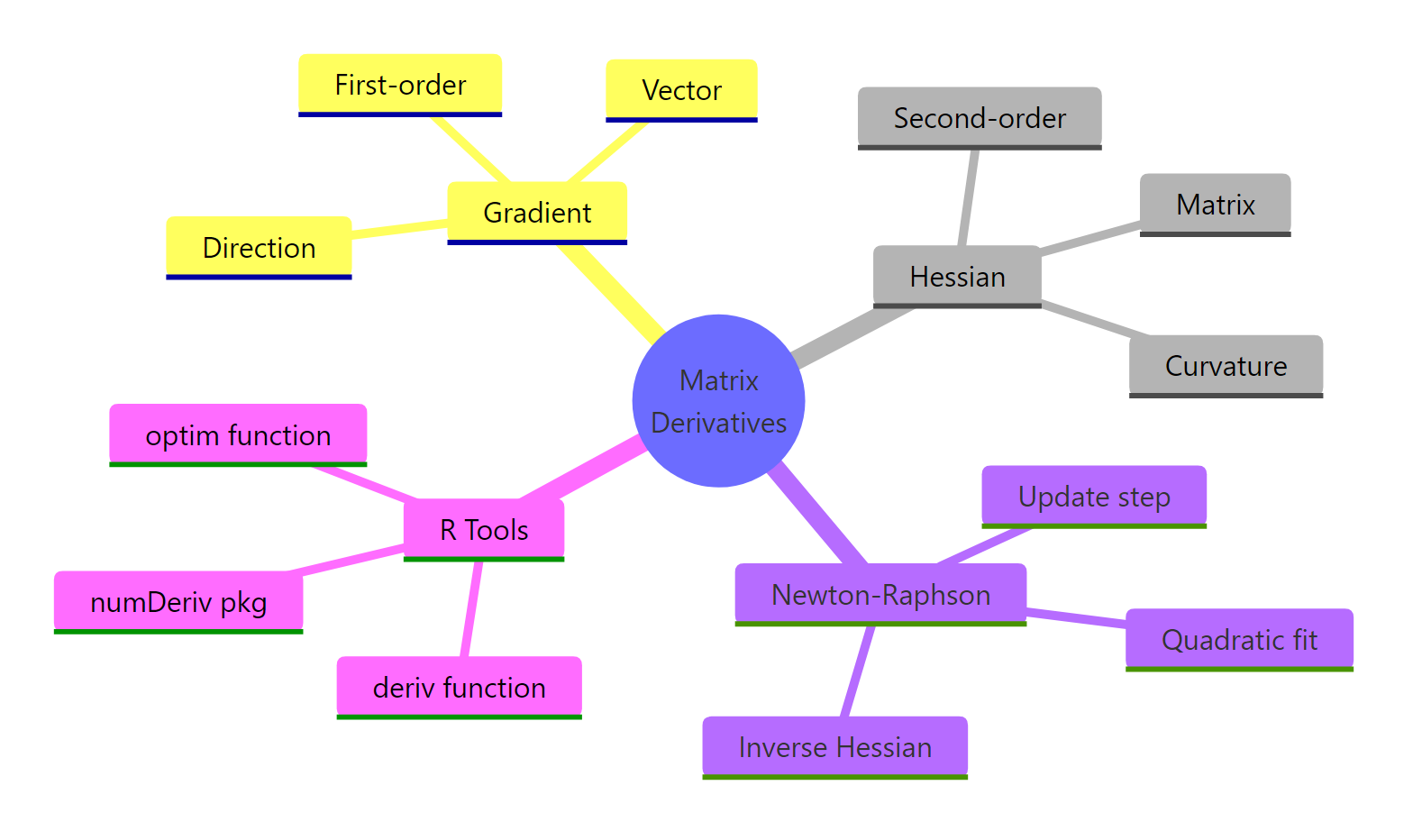
Overview of matrix derivatives and Newton-Raphson in R.

Figure 3: Overview of matrix derivatives and Newton-Raphson in R.

Concept	What it is	R tool
Gradient	Vector of first partial derivatives, $\nabla f$	`numDeriv::grad()`, `deriv()`
Hessian	Matrix of second partial derivatives, $H$	`numDeriv::hessian()`, `deriv(..., hessian = TRUE)`
Critical-point test	Eigenvalues of $H$	`eigen(H)$values`
Newton step	$\mathbf{x}_{k+1} = \mathbf{x}_k - H^{-1} \nabla f$	`solve(H, -g)`
Damped Newton	Scale step by $\gamma$ until $f$ decreases	Backtracking line search
Quasi-Newton fallback	BFGS approximates $H$ from gradients	`optim(method = "BFGS")`

Use deriv() when you have a formula, numDeriv for closures and black-box losses, pure Newton-Raphson when the Hessian is well-conditioned and the start is close, damped Newton when you might overshoot, and BFGS when you don't want to compute the Hessian at all.

References

R Core Team. Symbolic and Algorithmic Derivatives of Simple Expressions (?deriv documentation). Link
Gilbert, P. and Varadhan, R. numDeriv: Accurate Numerical Derivatives (CRAN package). Link
Nocedal, J. and Wright, S. Numerical Optimization, 2nd Edition. Springer (2006). Chapters 3 and 6 on Newton's method and quasi-Newton methods.
Wikipedia. Newton's method in optimization. Link
Peng, R. Advanced Statistical Computing, "The Newton Direction." Link
R Core Team. General-purpose Optimization (?optim documentation). Link
Givens, G. H. and Hoeting, J. A. Computational Statistics, 2nd Edition. Wiley (2013). Chapter on optimization.
Tibshirani, R. Newton's Method (Convex Optimization lecture notes, CMU 10-725). Link

Continue Learning

Maximum Likelihood Estimation in R, the most common Newton-Raphson use case in statistics, with optim() and mle() recipes.
Eigenvalues and Eigenvectors in R, covering the eigen() test we used to classify critical points in depth.
Solving Linear Systems in R, covering what solve(H, -g) is doing under the hood, including LU decomposition and condition numbers.