Spectral Decomposition in R: Diagonalization & Powers of Matrices

Spectral decomposition factors a symmetric matrix $A$ into $Q \Lambda Q^\top$, where $\Lambda$ holds the eigenvalues on the diagonal and the columns of $Q$ are orthonormal eigenvectors. That single factorisation lets you reconstruct $A$, raise it to any power in one shot, and read off its geometric structure.

What does spectral decomposition do?

The fastest way to understand spectral decomposition is to do it. We will build a small symmetric 3×3 matrix and feed it to eigen(). The eigenvalues come back as stretching factors, and the eigenvectors come back as the directions those stretches happen along. Once you have these two pieces, every other operation in this post is a one-line follow-up. Base R has everything we need, no extra packages.

RDecompose a symmetric matrix

set.seed(101) M <- matrix(rnorm(9), nrow = 3) A <- crossprod(M) # A = M^T M is guaranteed symmetric A #> [,1] [,2] [,3] #> [1,] 0.4985 0.4459 -0.2772 #> [2,] 0.4459 1.7991 -0.0625 #> [3,] -0.2772 -0.0625 0.7949 dec <- eigen(A) Q <- dec$vectors # eigenvectors as columns Lambda <- dec$values # eigenvalues as a numeric vector Lambda #> [1] 1.999 0.794 0.299

The matrix A is the symmetric product M^T M, a common way to manufacture a symmetric matrix from any starting matrix. Calling eigen(A) returns a list with two slots. The values slot is a vector of eigenvalues sorted from largest to smallest. The vectors slot is a matrix whose columns are the matching unit eigenvectors. Together they are the spectral decomposition: three numbers and three directions that completely describe how A acts on every vector in 3D space.

Key Insight

Eigenvectors are the axes the matrix stretches along, eigenvalues are how much it stretches. Any symmetric matrix is just three (or n) independent stretches along perpendicular axes, that is the entire content of the spectral theorem.

Try it: Pull the largest eigenvalue and its matching eigenvector out of dec. The eigenvalues come back already sorted in decreasing order, so this is a one-liner.

RYour turn: extract the top eigenpair

# your code here ex_top_val <- NULL ex_top_vec <- NULL ex_top_val ex_top_vec #> Expected: ex_top_val ~ 1.999 #> Expected: ex_top_vec is a length-3 unit vector

Click to reveal solution

RTop eigenpair solution

ex_top_val <- dec$values[1] ex_top_vec <- dec$vectors[, 1] ex_top_val #> [1] 1.999 ex_top_vec #> [1] -0.2856 -0.9362 0.2055

Explanation: eigen() always returns eigenvalues in decreasing order, so index [1] is the largest. The matching eigenvector is column 1 of $vectors.

How do you reconstruct A from Q and Λ?

The spectral theorem says $A = Q \Lambda Q^\top$ for any real symmetric matrix. Multiplying that out reconstructs A exactly, up to floating-point noise. The reason this formula is so clean is that for a symmetric matrix, the eigenvector matrix Q is orthogonal, which means $Q^{-1} = Q^\top$. We get to use a transpose where general matrices need a full inverse.

We will plug Q and Lambda from the previous block straight into the formula. Note that Lambda is a vector, so we wrap it with diag() to get the diagonal matrix the formula expects.

RReconstruct A from its decomposition

A_rebuilt <- Q %*% diag(Lambda) %*% t(Q) all.equal(A, A_rebuilt) #> [1] TRUE round(A_rebuilt, 4) #> [,1] [,2] [,3] #> [1,] 0.4985 0.4459 -0.2772 #> [2,] 0.4459 1.7991 -0.0625 #> [3,] -0.2772 -0.0625 0.7949

all.equal() is the right tolerance check for floating-point comparisons; == would fail on the last bit of every entry. The reconstruction matches A to machine precision. That confirms the decomposition is lossless, the three eigenvalues and three eigenvectors carry all of the information in the original 9 entries of A.

Tip

Always sanity-check orthogonality with crossprod(Q). For a symmetric matrix's eigenvector matrix, crossprod(Q) should equal the identity. If it does not, your input was not actually symmetric (a common bug when matrices were constructed from data with rounding).

Try it: Compute crossprod(Q) and round it to 6 decimal places. The result should be the 3×3 identity matrix.

RYour turn: confirm Q is orthogonal

ex_QtQ <- NULL # your code here round(ex_QtQ, 6) #> Expected: 3x3 identity

Click to reveal solution

ROrthogonality check solution

ex_QtQ <- crossprod(Q) round(ex_QtQ, 6) #> [,1] [,2] [,3] #> [1,] 1 0 0 #> [2,] 0 1 0 #> [3,] 0 0 1

Explanation: crossprod(Q) is shorthand for t(Q) %*% Q. For an orthogonal matrix, this is the identity by definition. Rounding hides the tiny floating-point drift that would otherwise show up in the off-diagonal entries.

How do you compute matrix powers in one shot?

This is the result that makes spectral decomposition genuinely useful. Once you have $A = Q \Lambda Q^\top$, raising A to any integer power k is

$$A^k = Q \Lambda^k Q^\top$$

and because $\Lambda$ is diagonal, $\Lambda^k$ is just the element-wise power on the diagonal, no matrix multiplication at all. That turns k - 1 matrix multiplies into one element-wise vector power plus two matrix multiplies, regardless of how big k is.

To see the payoff, we will compute $A^{10}$ two ways. First the naive way: chain ten copies of A together with Reduce() and %*%. Then the spectral way.

RCompute A^10 the slow way

A_pow_slow <- Reduce(`%*%`, replicate(10, A, simplify = FALSE)) round(A_pow_slow, 3) #> [,1] [,2] [,3] #> [1,] 97.05 359.29 -45.45 #> [2,] 359.29 1422.41 -125.99 #> [3,] -45.45 -125.99 35.62

Reduce() walks left to right multiplying ten copies of A. We picked 10 here because it is small enough to read but big enough that the entries blow up, eigenvalues greater than 1 dominate quickly.

RCompute A^10 via spectral decomposition

A_pow_fast <- Q %*% diag(Lambda^10) %*% t(Q) all.equal(A_pow_slow, A_pow_fast) #> [1] TRUE round(A_pow_fast, 3) #> [,1] [,2] [,3] #> [1,] 97.05 359.29 -45.45 #> [2,] 359.29 1422.41 -125.99 #> [3,] -45.45 -125.99 35.62

The two approaches agree to floating-point precision. The spectral form does the same job in three operations regardless of whether k is 10 or 10,000. That speedup matters most for fractional powers ($A^{1/2}$, the matrix square root) and negative powers ($A^{-1}$, the inverse), both of which become element-wise on the eigenvalues.

Warning

Watch for overflow and underflow with extreme powers. A small eigenvalue raised to a large k underflows to 0 and an eigenvalue greater than 1 raised to a large k overflows to Inf. If your matrix has eigenvalues spanning many orders of magnitude, work with log(Lambda) * k and exponentiate carefully, or use a numerically aware library like expm.

Try it: Compute $A^3$ via spectral decomposition and verify it matches A %*% A %*% A.

RYour turn: A^3 via spectral

ex_A_cube <- NULL # your code here all.equal(ex_A_cube, A %*% A %*% A) #> Expected: TRUE

Click to reveal solution

RA^3 spectral solution

ex_A_cube <- Q %*% diag(Lambda^3) %*% t(Q) all.equal(ex_A_cube, A %*% A %*% A) #> [1] TRUE

Explanation: Same formula as A^10, just with Lambda^3 on the diagonal. The cost is identical regardless of the exponent.

Does spectral decomposition work for non-symmetric matrices?

Yes, but with one important change. For a general (diagonalisable) matrix B, the formula becomes

$$B = V D V^{-1}$$

where the columns of V are still eigenvectors but they are not orthogonal anymore. That means we cannot replace $V^{-1}$ with $V^\top$, we have to compute the actual inverse with solve(). The matrix powers shortcut still works:

$$B^k = V D^k V^{-1}$$

Let's see this in action with an asymmetric matrix.

RDecompose an asymmetric matrix

B <- matrix(c(4, 1, 0, 2, 3, 0, 1, 0, 2), nrow = 3, byrow = TRUE) dec_B <- eigen(B) V <- dec_B$vectors D <- dec_B$values round(crossprod(V), 4) # NOT the identity #> [,1] [,2] [,3] #> [1,] 1.0000 0.7715 0.4923 #> [2,] 0.7715 1.0000 -0.4856 #> [3,] 0.4923 -0.4856 1.0000

crossprod(V) is clearly not the identity, which proves V is not orthogonal. So the symmetric trick t(V) will not give us the inverse. We have to use solve(V).

RReconstruct B and compute B^4

B_rebuilt <- V %*% diag(D) %*% solve(V) B_pow_fast <- V %*% diag(D^4) %*% solve(V) all.equal(B, B_rebuilt) #> [1] TRUE all.equal(B_pow_fast, B %*% B %*% B %*% B) #> [1] TRUE

Both checks pass. The decomposition still works, we just paid the cost of one explicit inverse instead of getting it for free from a transpose.

Note

Some matrices have complex eigenvalues, and that is normal. A 2D rotation matrix has eigenvalues $\cos\theta \pm i\sin\theta$. R's eigen() automatically returns complex types in that case, and the same V D V^{-1} formula still works, just with complex arithmetic. If you reconstruct and the imaginary parts are tiny noise, drop them with Re() after verifying.

Try it: Compute $B^2$ via spectral decomposition and verify it matches B %*% B.

RYour turn: B^2 via spectral

ex_B_sq <- NULL # your code here all.equal(ex_B_sq, B %*% B) #> Expected: TRUE

Click to reveal solution

RB^2 spectral solution

ex_B_sq <- V %*% diag(D^2) %*% solve(V) all.equal(ex_B_sq, B %*% B) #> [1] TRUE

Explanation: The non-symmetric formula is V D^k V^-1. We square the eigenvalues element-wise on the diagonal and use solve(V) for the inverse since V is not orthogonal here.

Practice Exercises

These capstone problems combine the concepts from above. Use distinct variable names with the my_ prefix so your work does not overwrite the tutorial state.

Exercise 1: Symmetric A^5 two ways

Build the symmetric matrix my_S <- crossprod(matrix(c(1, 2, 1, 0, 1, 1, 2, 0, 1), nrow = 3)). Compute my_S raised to the 5th power two ways: a matrix-multiply chain in my_pow_slow and a spectral computation in my_pow_fast. Verify they agree.

RExercise 1: symmetric power two ways

my_S <- crossprod(matrix(c(1, 2, 1, 0, 1, 1, 2, 0, 1), nrow = 3)) # Write your code below: my_pow_slow <- NULL my_pow_fast <- NULL all.equal(my_pow_slow, my_pow_fast) #> Expected: TRUE

Click to reveal solution

RExercise 1 solution

my_S <- crossprod(matrix(c(1, 2, 1, 0, 1, 1, 2, 0, 1), nrow = 3)) my_pow_slow <- Reduce(`%*%`, replicate(5, my_S, simplify = FALSE)) dec_S <- eigen(my_S) my_pow_fast <- dec_S$vectors %*% diag(dec_S$values^5) %*% t(dec_S$vectors) all.equal(my_pow_slow, my_pow_fast) #> [1] TRUE

Explanation: my_S is symmetric (built from crossprod), so the orthogonal-Q form applies and we use t() instead of solve(). Element-wise power on the eigenvalues replaces five matrix multiplies.

Exercise 2: Markov chain stationary distribution

Build the 2-state transition matrix my_P <- matrix(c(0.7, 0.3, 0.2, 0.8), nrow = 2, byrow = TRUE) (row 1 sums to 1, row 2 sums to 1). Decompose it, raise it to the 100th power spectrally, and read the stationary distribution off any row. The stationary distribution is the long-run probability of being in each state.

RExercise 2: Markov P^100 via spectral

my_P <- matrix(c(0.7, 0.3, 0.2, 0.8), nrow = 2, byrow = TRUE) # Write your code below, store the stationary distribution in my_pi: my_dec <- NULL my_P100 <- NULL my_pi <- NULL my_pi #> Expected: roughly c(0.4, 0.6)

Click to reveal solution

RExercise 2 solution

my_P <- matrix(c(0.7, 0.3, 0.2, 0.8), nrow = 2, byrow = TRUE) my_dec <- eigen(my_P) my_P100 <- my_dec$vectors %*% diag(my_dec$values^100) %*% solve(my_dec$vectors) my_pi <- my_P100[1, ] round(Re(my_pi), 4) #> [1] 0.4 0.6

Explanation: my_P is not symmetric, so we use solve(). After many steps every row of $P^{100}$ converges to the same row vector, that vector is the stationary distribution. We wrap with Re() because numerical drift can leave a tiny imaginary part.

Complete Example: Markov chain steady state via diagonalisation

Here is the workflow end-to-end. We will model weather transitions in three states (Sunny, Cloudy, Rainy), find $P^{50}$ via spectral decomposition, and confirm the steady-state distribution two different ways. The transition matrix is non-symmetric, so this is the V D V^-1 form we just learned.

RThree-state weather Markov chain

trans <- matrix(c(0.80, 0.15, 0.05, # from Sunny 0.30, 0.55, 0.15, # from Cloudy 0.20, 0.30, 0.50), # from Rainy nrow = 3, byrow = TRUE) rownames(trans) <- colnames(trans) <- c("Sunny", "Cloudy", "Rainy") dec_T <- eigen(trans) V_T <- dec_T$vectors D_T <- dec_T$values round(D_T, 4) #> [1] 1.0000 0.4854 0.3646

The largest eigenvalue is exactly 1, every valid transition matrix has this property because rows sum to 1. The other eigenvalues are all less than 1 in absolute value, so their powers shrink to zero. After enough steps, only the eigenvalue-1 component survives, and that survivor is the steady state.

RPower the chain forward 50 steps

T50 <- V_T %*% diag(D_T^50) %*% solve(V_T) round(Re(T50), 4) #> Sunny Cloudy Rainy #> Sunny 0.5634 0.2958 0.1408 #> Cloudy 0.5634 0.2958 0.1408 #> Rainy 0.5634 0.2958 0.1408

Every row is identical. That tells us the Markov chain has fully converged: starting from any initial state, the probability of being in Sunny / Cloudy / Rainy after 50 steps is the same. We can read the stationary distribution pi straight off any row.

RRead off the steady state and cross-check

pi_steady <- Re(T50[1, ]) pi_steady #> Sunny Cloudy Rainy #> 0.5634 0.2958 0.1408 # Cross-check: pi should satisfy pi %*% trans == pi round(pi_steady %*% trans, 4) #> Sunny Cloudy Rainy #> 0.5634 0.2958 0.1408

The fixed-point equation $\pi P = \pi$ holds, which is the defining property of a stationary distribution. The chain spends about 56% of its time in Sunny, 30% in Cloudy, and 14% in Rainy, and we got there by raising the transition matrix to a high power in three lines, no simulation required.

Summary

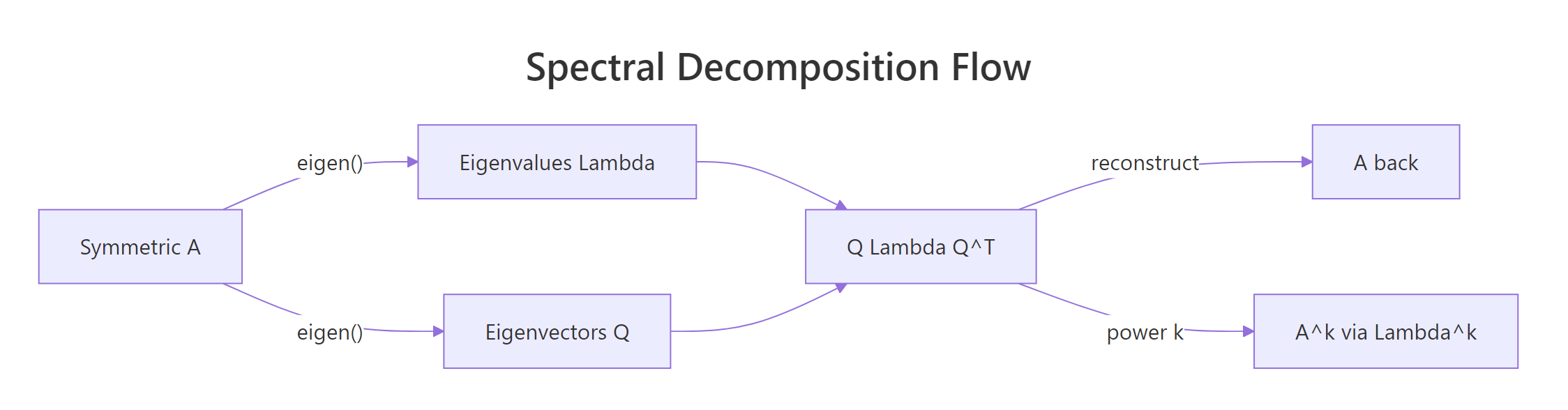
Spectral decomposition flow: A passes through eigen() to produce Lambda and Q, which recombine into Q Lambda Q^T to either reconstruct A or compute any power.

Figure 1: Spectral decomposition turns a symmetric matrix A into three pieces, Q, Λ, Qᵀ, that recombine to give back A or any of its powers.

Concept	Formula	R idiom
Symmetric reconstruction	$A = Q \Lambda Q^\top$	`Q %% diag(Lambda) %% t(Q)`
Matrix power (symmetric)	$A^k = Q \Lambda^k Q^\top$	`Q %% diag(Lambda^k) %% t(Q)`
Non-symmetric reconstruction	$B = V D V^{-1}$	`V %% diag(D) %% solve(V)`
Markov stationary distribution	row of $P^k$ for large $k$	any row of `V %% diag(D^k) %% solve(V)`

The single mental model: spectral decomposition = independent stretches along independent axes. Reconstruction is regrouping those pieces. Powering is element-wise on the diagonal of stretches. Symmetric matrices buy you a free transpose where general ones need a real inverse.

References

R Core Team. eigen, Spectral Decomposition of a Matrix. R base documentation. Link
Wikipedia. Eigendecomposition of a matrix. Link
Friendly, M. matlib vignette: Eigenvalues and Spectral Decomposition. Link
Wilkinson, R. MATH3030 Multivariate Statistics §3.2: Spectral / eigen decomposition. Link
Strang, G. Introduction to Linear Algebra, 5th edition. Wellesley-Cambridge Press (2016). Chapter 6: Eigenvalues and Eigenvectors.
Trefethen, L. N., and Bau, D. Numerical Linear Algebra. SIAM (1997). Lecture 24: Eigenvalue Algorithms.

Continue Learning

Eigenvalues & Eigenvectors in R: eigen(), Why They Power PCA & More. The prerequisite for this post: what eigen() returns, what eigenvalues mean, and how PCA uses them.
Solving Linear Systems in R: solve(), qr() & Least Squares Solutions. The companion factorisation topic, LU and QR decompositions for solving $Ax = b$.
Matrix Operations in R: Create, Multiply, Invert & Transpose for Statistics. Base R matrix algebra primer if %*%, t(), or solve() still feel new.

Spectral Decomposition in R: Diagonalization & Powers of Matrices

What does spectral decomposition do?

How do you reconstruct A from Q and Λ?

How do you compute matrix powers in one shot?

Does spectral decomposition work for non-symmetric matrices?

Practice Exercises

Exercise 1: Symmetric A^5 two ways

Exercise 2: Markov chain stationary distribution

Complete Example: Markov chain steady state via diagonalisation

Summary

References

Continue Learning

Related Tutorials