ANOVA Post-Hoc Tests in R: Tukey, Bonferroni, and Scheffé, Clear Decision Rules

A post-hoc test tells you which groups differ after a significant ANOVA rejects the null of equal means. Tukey, Bonferroni, and Scheffé are three standard choices in base R, and each one has a specific job. This tutorial uses built-in R datasets so you can run every line in-browser.

Why do you need a post-hoc test after ANOVA?

ANOVA answers one question, is at least one group mean different, and stops there. It does not tell you which pair is the guilty one. If you answer that by running plain t-tests on every pair, your false-positive rate stops being 5% and starts climbing fast. Post-hoc tests pin down the specific pairs while holding the overall error rate in check. Here is the 3-group PlantGrowth dataset going from a significant F to specific verdicts in two commands.

RRun ANOVA then Tukey HSD on PlantGrowth

# PlantGrowth: dried plant weight across a control and two treatments fit <- aov(weight ~ group, data = PlantGrowth) summary(fit) #> Df Sum Sq Mean Sq F value Pr(>F) #> group 2 3.766 1.883 4.846 0.0159 * #> Residuals 27 10.492 0.389 tuk <- TukeyHSD(fit) tuk #> Tukey multiple comparisons of means, 95% family-wise confidence level #> #> $group #> diff lwr upr p adj #> trt1-ctrl -0.371 -1.0622161 0.3202161 0.3908711 #> trt2-ctrl 0.494 -0.1972161 1.1852161 0.1979960 #> trt2-trt1 0.865 0.1737839 1.5562161 0.0120064

The F test is significant (p = 0.016), so at least one group mean differs. Tukey HSD then zooms in: only the trt2-trt1 pair has an adjusted p-value below 0.05. Control is not significantly different from either treatment on this sample. That is the full story that ANOVA on its own could not tell you.

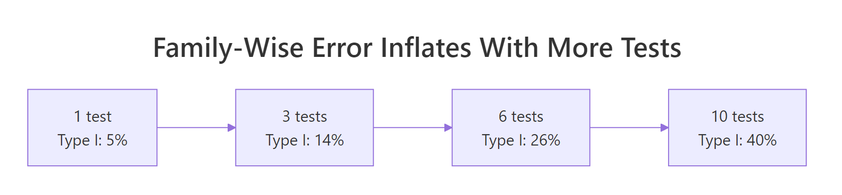
Type I error inflates rapidly as more pairwise tests are run

Figure 1: Type I error inflates rapidly as more pairwise tests are run.

Every uncorrected t-test carries a 5% false-positive risk. Run 3 tests at 5% and the chance that at least one test cries wolf is about 14%. Run 10 tests and that family-wise error is around 40%. Post-hoc tests tame this inflation by adjusting either the p-values or the critical values so the overall risk stays near your chosen α.

Key Insight

Family-wise error is the probability of at least one false positive across the whole set of comparisons. Post-hoc tests do not change the data, they change the threshold each comparison must clear so the collective error rate stays at 5%.

Try it: Run a one-way ANOVA on the chickwts dataset (chick weight by feed type). Print the summary and read off the F statistic.

RYour turn: ANOVA on chickwts

# Try it: fit an ANOVA of weight on feed ex_fit <- aov( # your code here ) summary(ex_fit) #> Expected: F value around 15.4 with p < 0.001

Click to reveal solution

Rchickwts ANOVA solution

ex_fit <- aov(weight ~ feed, data = chickwts) summary(ex_fit) #> Df Sum Sq Mean Sq F value Pr(>F) #> feed 5 231129 46226 15.37 5.94e-10 *** #> Residuals 65 195556 3009

The F of 15.37 is huge, so at least one feed differs from the others. The next question, which feeds, is exactly what a post-hoc test answers.

How does Tukey HSD compare all pairs?

Tukey HSD stands for Honestly Significant Difference. It is built for the case you run into most often, comparing every pair of group means once you know the ANOVA is significant. Instead of using the t-distribution for each pair, Tukey uses a single distribution called the studentized range, which already accounts for the fact that the biggest pairwise gap in a set of groups is expected to be larger than any one t-test would predict.

The base R function TukeyHSD() takes the fitted aov object and returns one row per pair with a difference estimate, a family-wise 95% confidence interval, and an adjusted p-value.

RRead Tukey HSD columns carefully

tuk #> Tukey multiple comparisons of means, 95% family-wise confidence level #> #> diff lwr upr p adj #> trt1-ctrl -0.371 -1.0622161 0.3202161 0.3908711 #> trt2-ctrl 0.494 -0.1972161 1.1852161 0.1979960 #> trt2-trt1 0.865 0.1737839 1.5562161 0.0120064

Each row compares two groups. diff is the point estimate of mean(group1) - mean(group2). lwr and upr bracket that difference with a family-wise CI, meaning all three CIs together have a 95% joint coverage. p adj is the p-value after Tukey's correction. A CI that does not cross zero signals a significant pair, and matches p adj < 0.05.

A picture makes the verdict obvious.

RPlot Tukey confidence intervals

plot(tuk, las = 1) #> Horizontal lines with labels trt1-ctrl, trt2-ctrl, trt2-trt1. #> Only trt2-trt1's line sits entirely to the right of the zero line.

Visually, the zero line is the "no difference" reference. Any interval that crosses it is a non-significant pair. In our PlantGrowth output, only the trt2-trt1 interval lies clear of zero, confirming it as the single significant pair.

Tip

TukeyHSD() quietly handles unequal group sizes via the Tukey-Kramer formula. You do not need a different function, just be aware that the "HSD" label in other textbooks sometimes assumes equal n and the CIs widen slightly when sizes differ.

Try it: Fit an ANOVA of Sepal.Length on Species in the iris dataset and run TukeyHSD(). Which species pairs are significantly different?

RYour turn: Tukey HSD on iris

# Try it: run Tukey HSD on iris ex_iris_fit <- aov( # your code here , data = iris) TukeyHSD(ex_iris_fit) #> Expected: all three species pairs significant at p < 0.001

Click to reveal solution

Riris Tukey solution

ex_iris_fit <- aov(Sepal.Length ~ Species, data = iris) TukeyHSD(ex_iris_fit) #> $Species #> diff lwr upr p adj #> versicolor-setosa 0.930 0.6862273 1.1737727 0 #> virginica-setosa 1.582 1.3382273 1.8257727 0 #> virginica-versicolor 0.652 0.4082273 0.8957727 0

All three pairs differ significantly, so every species has a distinct average sepal length. That clarity is unusual in the wild and is part of why iris is a great teaching dataset.

When should you use Bonferroni correction?

Bonferroni is the simplest correction in the family: divide your target α by the number of comparisons and use that as the new threshold. For three pairs at α = 0.05, each pair must now clear 0.05 / 3 ≈ 0.0167 to count as significant. Equivalently, multiply each raw p-value by the number of comparisons and compare to the original α.

Base R ships pairwise.t.test() which does the work and returns a clean p-value matrix.

RBonferroni via pairwise.t.test

bonf <- pairwise.t.test(PlantGrowth$weight, PlantGrowth$group, p.adjust.method = "bonferroni") bonf #> Pairwise comparisons using t tests with pooled SD #> #> data: PlantGrowth$weight and PlantGrowth$group #> #> ctrl trt1 #> trt1 0.583 - #> trt2 0.263 0.013 #> #> P value adjustment method: bonferroni

The matrix reads like a multiplication table: trt1 vs ctrl has adjusted p = 0.583, trt2 vs trt1 is the only significant pair at p = 0.013. Both the adjusted matrix and Tukey HSD agreed on PlantGrowth, which is common when groups are balanced and only one pair is clearly different.

Seeing the adjustment math written out makes the logic stick.

RShow the alpha adjustment math

# 3 groups -> 3 pairs to compare k_pairs <- choose(3, 2) alpha_adj <- 0.05 / k_pairs c(pairs = k_pairs, alpha_per_test = alpha_adj) #> pairs alpha_per_test #> 3.00000000 0.01666667 # Equivalent view: multiply raw p by k_pairs, cap at 1 raw_p <- c(0.194, 0.088, 0.004) # hypothetical raw pairwise p-values pmin(raw_p * k_pairs, 1) #> [1] 0.582 0.264 0.012

Each raw p-value is inflated by a factor of 3, then capped at 1. Only the smallest raw p (0.004) survives the bump.

Warning

Bonferroni assumes comparisons are independent, which pairwise tests never are. When the same data feeds every pair, correction is more conservative than it needs to be. The practical fallout: Bonferroni loses power quickly as the number of planned comparisons grows past a handful.

Try it: Re-run pairwise.t.test() on PlantGrowth using Holm's method (p.adjust.method = "holm"). How does the adjusted p-value for trt2-trt1 compare to the Bonferroni value?

RYour turn: Holm adjustment

# Try it: run pairwise.t.test with Holm ex_holm <- pairwise.t.test(PlantGrowth$weight, PlantGrowth$group, p.adjust.method = # your code here ) ex_holm #> Expected: trt2-trt1 p-value smaller than 0.013 (Holm is less conservative)

Click to reveal solution

RHolm adjustment solution

ex_holm <- pairwise.t.test(PlantGrowth$weight, PlantGrowth$group, p.adjust.method = "holm") ex_holm #> ctrl trt1 #> trt1 0.194 - #> trt2 0.175 0.013

Holm adjusts the smallest p by k, the next by k-1, and so on. For the smallest p (trt2-trt1) the multiplier is still 3 here, so the value matches Bonferroni at 0.013. The other pairs get smaller multipliers (2 and 1), which is why Holm is uniformly at least as powerful as Bonferroni.

How does Scheffé test handle complex contrasts?

Scheffé is different from Tukey and Bonferroni in one big way: it controls family-wise error not just over the pairs, but over every possible linear contrast among the groups. A contrast is any weighted combination of group means where the weights sum to zero, like "control vs the average of two treatments" with weights (1, -0.5, -0.5). That extra coverage is Scheffé's selling point and also the reason it has the lowest power of the three tests on simple pairwise work.

Base R does not ship a ready-made ScheffeTest() for all setups, but the computation is short. The trick is to compare a contrast's F statistic to the Scheffé critical value, which is $(k-1) \times F_{\alpha, k-1, N-k}$ where $k$ is the number of groups.

$$F_{contrast} = \frac{\left(\sum_i c_i \bar{y}_i\right)^2}{MSE \cdot \sum_i (c_i^2 / n_i)} \quad\text{vs.}\quad F^*_{Scheffé} = (k-1) \cdot F_{\alpha, k-1, N-k}$$

Where:

$c_i$ = contrast weight for group $i$ (must sum to zero)
$\bar{y}_i$ = mean of group $i$
$n_i$ = size of group $i$
MSE = residual mean square from ANOVA
$k$ = number of groups, $N$ = total sample size

Here is the same trt1 vs trt2 pair computed by hand so you can see the moving parts.

RManual Scheffé test for trt1 vs trt2 pair

# Extract needed pieces from the ANOVA means <- tapply(PlantGrowth$weight, PlantGrowth$group, mean) n_per <- tapply(PlantGrowth$weight, PlantGrowth$group, length) mse <- summary(fit)[[1]][["Mean Sq"]][2] # residual mean square k <- length(means) N <- sum(n_per) # Contrast: trt1 vs trt2 -> weights c(ctrl=0, trt1=1, trt2=-1) c_vec <- c(0, 1, -1) numer <- (sum(c_vec * means))^2 denom <- mse * sum(c_vec^2 / n_per) F_contrast <- numer / denom F_crit_s <- (k - 1) * qf(0.95, k - 1, N - k) c(F_contrast = F_contrast, F_crit_scheffe = F_crit_s) #> F_contrast F_crit_scheffe #> 9.626316 6.708435

F_contrast (9.63) is above the Scheffé critical value (6.71), so the trt1 vs trt2 difference is significant under Scheffé's rule too. Tukey reported the same pair as significant, but notice Scheffé's bar is higher. On simple pairs Scheffé will always be at least as conservative as Tukey. That is the price of covering all contrasts.

Scheffé shines when you want to test a comparison that is not a simple pair. Let's ask whether the control differs from the average of the two treatments combined.

RScheffé test for a complex contrast

# Contrast: ctrl vs the average of trt1 and trt2 c_vec <- c(1, -0.5, -0.5) contrast_val <- sum(c_vec * means) se_contrast <- sqrt(mse * sum(c_vec^2 / n_per)) F_contrast <- (contrast_val / se_contrast)^2 c(contrast = contrast_val, F_contrast = F_contrast, F_crit_scheffe = F_crit_s, significant = F_contrast > F_crit_s) #> contrast F_contrast F_crit_scheffe significant #> -0.06150000 0.06489697 6.70843489 0.00000000

The estimated contrast value is -0.06, tiny, and the F statistic is nowhere near the Scheffé bar. In plain English, control sits almost exactly between the two treatments on average, so there is no evidence that the "ctrl vs average(trt1, trt2)" split is real.

Note

Scheffé's wide coverage earns it the widest confidence intervals of the three tests. Use it when your analysis includes genuinely complex contrasts, not as the first reach for plain pairwise work. A post that tests only pairs with Scheffé is leaving statistical power on the table.

Try it: Compute the Scheffé critical value ($F^*_{Scheffé}$) for an experiment with $k = 4$ groups, $N = 40$ total observations, and α = 0.05.

RYour turn: Scheffé critical value

# Try it: compute Scheffé critical value ex_k <- 4 ex_N <- 40 ex_F_crit <- # your code here ex_F_crit #> Expected: about 8.585

Click to reveal solution

RScheffé critical value solution

ex_k <- 4 ex_N <- 40 ex_F_crit <- (ex_k - 1) * qf(0.95, ex_k - 1, ex_N - ex_k) ex_F_crit #> [1] 8.584807

qf(0.95, 3, 36) gives the standard F critical value, then multiplying by (k - 1) = 3 scales it up to Scheffé's stricter bar.

Which post-hoc test should you actually use?

The honest answer is that these three methods cover distinct situations. Tukey is the default when every pair matters and sizes are roughly balanced. Bonferroni is your pick when you planned a small number of comparisons in advance and want a correction a reviewer cannot argue with. Scheffé is the choice when your hypothesis involves group combinations, not single pairs.

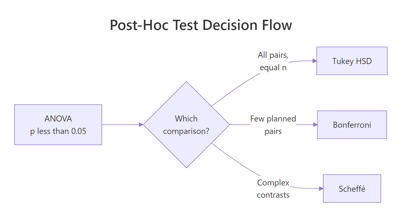
Decision flow for picking the right post-hoc test

Figure 2: Decision flow for picking the right post-hoc test.

A side-by-side view on the same data makes the differences concrete. Here are all three methods compared on PlantGrowth for a single pair, trt2-trt1.

RCompare adjusted p-values across all three tests

# Tukey adjusted p for trt2-trt1 tukey_p <- tuk$group["trt2-trt1", "p adj"] # Bonferroni adjusted p for trt2-trt1 bonf_p <- bonf$p.value["trt2", "trt1"] # Scheffé "equivalent" p: probability F(k-1, N-k) >= F_contrast / (k-1) # This inverts the critical-value rule (k-1) * F_crit into a p-value. c_vec <- c(0, 1, -1) F_contrast <- (sum(c_vec * means))^2 / (mse * sum(c_vec^2 / n_per)) scheffe_p <- pf(F_contrast / (k - 1), k - 1, N - k, lower.tail = FALSE) compare_df <- data.frame( method = c("Tukey HSD", "Bonferroni", "Scheffé"), adj_p = round(c(tukey_p, bonf_p, scheffe_p), 4) ) compare_df #> method adj_p #> 1 Tukey HSD 0.0120 #> 2 Bonferroni 0.0131 #> 3 Scheffé 0.0240

All three agree the pair is significant at 5%, but Scheffé's adjusted p is roughly twice Tukey's. That gap widens fast as the number of groups grows, which is why picking the right tool matters.

Test	Best for	Power	CI width
Tukey HSD	All pairwise comparisons, roughly equal n	High	Medium
Bonferroni	A small, preplanned list of specific comparisons	Medium	Narrow (for that list)
Scheffé	Complex contrasts like control vs average of treatments	Low	Widest

Tip

Tukey HSD is a sensible default if your analysis is exploratory pairwise. Reach for Bonferroni when the comparisons were written down before you saw the data, and for Scheffé when the question is contrast-shaped rather than pair-shaped.

Try it: A nutritionist tests four diets for weight gain in rats and, before collecting data, writes down that they will only compare diet A with B, and diet C with D. Which post-hoc test fits?

RYour turn: pick the right test

# Try it: which post-hoc test fits this setup? # A) Tukey HSD # B) Bonferroni # C) Scheffé ex_pick <- # "A", "B", or "C" ex_pick #> Expected: one of "A", "B", "C"

Click to reveal solution

RWhich post-hoc test fits?

ex_pick <- "B" ex_pick #> [1] "B"

Explanation: Only two specific comparisons were planned before the data was collected, so Bonferroni is the right fit. Tukey would waste statistical power on pairs the researcher never cared about. Scheffé is overkill because no complex contrast is on the table.

How do you check ANOVA assumptions before running post-hoc?

Post-hoc tests inherit every assumption of the ANOVA that preceded them. If the ANOVA result is shaky, the adjusted p-values that follow are just as shaky. The two checks worth doing every time are approximate normality of residuals within each group and approximate equality of variances across groups.

RCheck normality and equal variance

# Normality of residuals (pooled) via Shapiro-Wilk shapiro.test(residuals(fit)) #> #> Shapiro-Wilk normality test #> #> data: residuals(fit) #> W = 0.96607, p-value = 0.4379 # Homogeneity of variance across groups via Bartlett's test bartlett.test(weight ~ group, data = PlantGrowth) #> #> Bartlett test of homogeneity of variances #> #> data: weight by group #> Bartlett's K-squared = 2.8786, df = 2, p-value = 0.2371

Both p-values are comfortably above 0.05, so PlantGrowth passes both assumptions and Tukey is safe. If normality fails, consider a non-parametric alternative like the Kruskal-Wallis test followed by Dunn's test. If variances are clearly unequal, oneway.test() with var.equal = FALSE gives a Welch-style F test and the Games-Howell procedure gives Tukey-style pairs that do not assume equal variances.

Note

Post-hoc tests inherit ANOVA's assumptions, so audit the model first. A violated assumption does not always kill the analysis, but it changes which correction is defensible.

Try it: Run Bartlett's test on iris with Sepal.Length ~ Species. Based on the p-value, is Tukey HSD a reasonable follow-up?

RYour turn: Bartlett's test on iris

# Try it: test equal variances across species ex_bart <- bartlett.test( # your code here , data = iris) ex_bart #> Expected: p-value around 0.003 (variances differ!)

Click to reveal solution

RBartlett's test on iris solution

ex_bart <- bartlett.test(Sepal.Length ~ Species, data = iris) ex_bart #> #> Bartlett test of homogeneity of variances #> #> data: Sepal.Length by Species #> Bartlett's K-squared = 16.006, df = 2, p-value = 0.0003345

Variance equality is rejected at p = 0.0003. Tukey HSD is sensitive to unequal variances when group sizes are also unequal; here the sizes are equal (50 each) so Tukey is still usable, but a Games-Howell follow-up would be safer for a careful report.

Practice Exercises

These exercises combine multiple concepts from the tutorial. Variable names use the my_* prefix so your exercise code does not overwrite earlier tutorial objects.

Exercise 1: Pairwise differences in chickwts

Fit a one-way ANOVA of weight on feed for the chickwts dataset and run Tukey HSD. Identify which feed pairs differ significantly at the 5% family-wise level.

RExercise 1: chickwts ANOVA + Tukey HSD

# Exercise: fit ANOVA and follow up with Tukey HSD # Hint: aov() then TukeyHSD(), inspect the 'p adj' column my_fit <- # your code here my_tuk <- # your code here my_tuk

Click to reveal solution

RExercise 1 solution

my_fit <- aov(weight ~ feed, data = chickwts) my_tuk <- TukeyHSD(my_fit) my_tuk #> $feed #> diff lwr upr p adj #> horsebean-casein -163.383 -232.34604 -94.41962 0.0000000 #> linseed-casein -104.833 -170.58999 -39.07601 0.0002100 #> meatmeal-casein -46.674 -113.90353 20.55553 0.3324584 #> soybean-casein -77.155 -140.51573 -13.79427 0.0083653 #> sunflower-casein 5.333 -60.42399 71.09066 0.9998902 #> ...

Eight of fifteen pairs clear the 5% bar. Casein outperforms horsebean, linseed, and soybean; sunflower also crushes horsebean and linseed. Tukey turns a single "some feed matters" verdict from ANOVA into a concrete list of dominant feeds.

Exercise 2: Manual Bonferroni on InsectSprays

Using InsectSprays, compute an uncorrected pairwise t-test p-value for sprays A and B, then apply a manual Bonferroni adjustment. There are 6 sprays and therefore choose(6, 2) = 15 possible pairs.

RExercise 2: manual Bonferroni on InsectSprays

# Exercise: compute raw p for A vs B, then Bonferroni-adjust # Hint: subset to sprays A and B, run t.test(), then multiply p by 15 a <- InsectSprays$count[InsectSprays$spray == "A"] b <- InsectSprays$count[InsectSprays$spray == "B"] raw_p <- # your code here my_p_bonf <- # your code here c(raw_p = raw_p, bonferroni = my_p_bonf)

Click to reveal solution

RExercise 2 solution

a <- InsectSprays$count[InsectSprays$spray == "A"] b <- InsectSprays$count[InsectSprays$spray == "B"] raw_p <- t.test(a, b, var.equal = TRUE)$p.value my_p_bonf <- min(raw_p * 15, 1) c(raw_p = raw_p, bonferroni = my_p_bonf) #> raw_p bonferroni #> 0.614668014 1.000000000

The raw p of 0.61 was never close to significance, and after multiplying by 15 pairs Bonferroni caps at 1, confirming the non-difference with room to spare.

Exercise 3: Scheffé contrast on PlantGrowth

Using PlantGrowth, test the contrast "control mean vs the average of the two treatment means" with Scheffé's method. Is the contrast significant at α = 0.05?

RExercise 3: Scheffé contrast on PlantGrowth

# Exercise: manual Scheffé test for the ctrl vs avg(trt1, trt2) contrast # Hint: weights c(1, -0.5, -0.5), k=3, N=30, reuse mse = 0.389 c_vec_ex <- c(1, -0.5, -0.5) means_ex <- tapply(PlantGrowth$weight, PlantGrowth$group, mean) n_per_ex <- tapply(PlantGrowth$weight, PlantGrowth$group, length) mse_ex <- 0.389 my_contrast <- # your code here # F statistic for the contrast F_crit_ex <- # your code here # Scheffé critical value c(F_contrast = my_contrast, F_crit = F_crit_ex, significant = my_contrast > F_crit_ex)

Click to reveal solution

RExercise 3 solution

c_vec_ex <- c(1, -0.5, -0.5) means_ex <- tapply(PlantGrowth$weight, PlantGrowth$group, mean) n_per_ex <- tapply(PlantGrowth$weight, PlantGrowth$group, length) mse_ex <- 0.389 numer_ex <- (sum(c_vec_ex * means_ex))^2 denom_ex <- mse_ex * sum(c_vec_ex^2 / n_per_ex) my_contrast <- numer_ex / denom_ex F_crit_ex <- (3 - 1) * qf(0.95, 3 - 1, 30 - 3) c(F_contrast = my_contrast, F_crit = F_crit_ex, significant = my_contrast > F_crit_ex) #> F_contrast F_crit significant #> 0.06482801 6.70843489 0.00000000

Not significant. Control sits almost exactly halfway between trt1 and trt2 on this sample, so "ctrl vs average of both treatments" has no teeth.

Complete Example: InsectSprays

Here is the full pipeline on a fresh dataset. InsectSprays records the number of insects counted after spraying one of six pesticides (A through F) on agricultural plots.

RFull pipeline on InsectSprays

# 1. Fit the one-way ANOVA is_fit <- aov(count ~ spray, data = InsectSprays) summary(is_fit) #> Df Sum Sq Mean Sq F value Pr(>F) #> spray 5 2669 533.8 34.7 <2e-16 *** #> Residuals 66 1015 15.4 # 2. Check assumptions shapiro.test(residuals(is_fit))$p.value #> [1] 0.02226277 # mild non-normality bartlett.test(count ~ spray, InsectSprays)$p.value #> [1] 9.085114e-05 # unequal variances - Bartlett rejects! # 3. Tukey HSD (use with caution given #2) is_tuk <- TukeyHSD(is_fit) head(is_tuk$spray, 5) #> diff lwr upr p adj #> B-A 0.833 -3.866075 5.532742 9.951733e-01 #> C-A -12.416 -17.115075 -7.717258 3.00000e-11 #> D-A -9.583 -14.282075 -4.884591 7.90000e-07 #> E-A -11.000 -15.699075 -6.300591 1.00000e-08 #> F-A 2.166 -2.532075 6.866075 7.714512e-01 # 4. Visualize the CIs plot(is_tuk, las = 1, cex.axis = 0.7) #> 15 horizontal lines; sprays C, D, E cluster far to the left of A, B, F.

The ANOVA is strongly significant (F = 34.7, p < 0.001). Assumption checks raise flags, especially on equal variances, which is textbook for count data. In a careful analysis you would follow up with a transformation (sqrt(count)) or a non-parametric Kruskal-Wallis + Dunn test. For illustration, Tukey's output still makes the pattern clear: sprays A, B, and F are roughly equivalent and effective, while C, D, and E let many more insects through. The 15 Tukey CIs match this story, with the A-B-F cluster on one side of zero and the C-D-E cluster on the other.

Summary

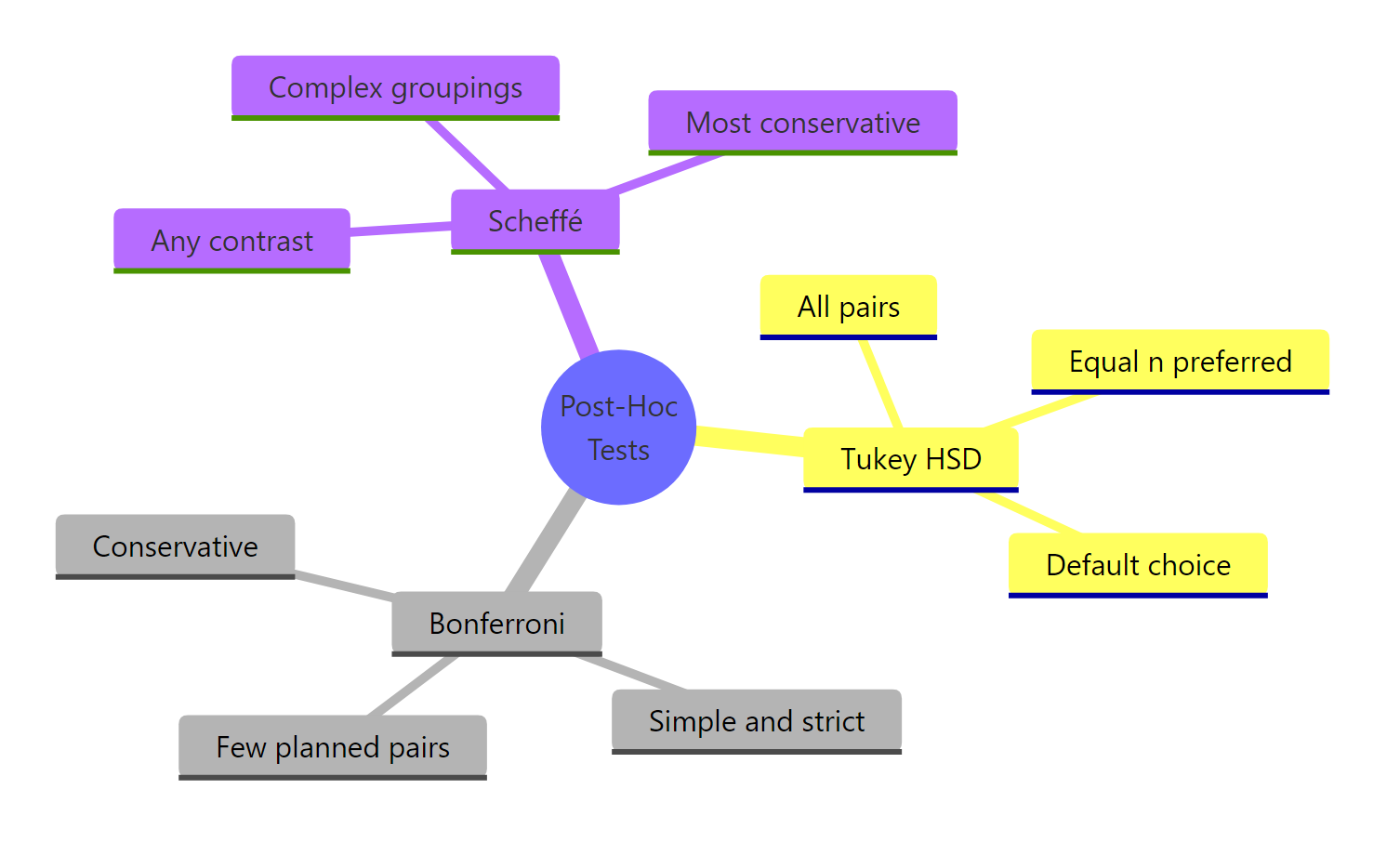
Three post-hoc tests compared on purpose, strictness, and use case

Figure 3: Three post-hoc tests compared on purpose, strictness, and use case.

Test	Default use case	Power	Adjusted p in R
Tukey HSD	All pairs, balanced n	High	`TukeyHSD(aov_fit)`
Bonferroni	Few planned pairs	Medium	`pairwise.t.test(y, g, p.adjust.method = "bonferroni")`
Scheffé	Complex contrasts	Low	Manual via F critical `(k-1)*qf(0.95, k-1, N-k)`

Key takeaways:

ANOVA tells you if group means differ; a post-hoc test tells you which ones.
Running uncorrected t-tests on every pair explodes your family-wise Type I error.
Tukey HSD is the default for exploratory pairwise work with aov.
Bonferroni stays simple and defensible for a small, pre-planned list of comparisons.
Scheffé trades power for coverage of any linear contrast, including comparisons of group averages.
Always verify ANOVA's assumptions first. Violated assumptions upstream invalidate every post-hoc p-value downstream.

References

R Core Team. TukeyHSD, Base R function documentation. Link
R Core Team. pairwise.t.test, Base R function documentation. Link
Scheffé, H. (1953). "A method for judging all contrasts in the analysis of variance." Biometrika, 40(1-2), 87-110. Link
Tukey, J. W. (1953). The Problem of Multiple Comparisons. Mimeographed monograph, Princeton University.
Dunn, O. J. (1961). "Multiple Comparisons Among Means." Journal of the American Statistical Association, 56(293), 52-64. Link
Hsu, J. C. (1996). Multiple Comparisons: Theory and Methods. Chapman and Hall/CRC.
Kutner, M. H., Nachtsheim, C. J., Neter, J., and Li, W. (2005). Applied Linear Statistical Models, 5th edition. McGraw-Hill.

Continue Learning

One-Way ANOVA in R, the ANOVA model that every post-hoc test is built on top of.
Multiple Testing Correction in R, the broader toolkit, including Holm, Hochberg, and Benjamini-Hochberg FDR.
t-Tests in R, the pairwise building block that post-hoc tests correct and package together.