DuckDB in R: Query 100 Million Rows on Your Laptop in Under 2 Seconds

DuckDB is an in-process analytical database that runs inside your R session, no server, no setup. It queries CSVs, Parquet files, and R data frames directly with SQL or dplyr syntax, and it does so fast enough to handle datasets that crash most tools.

Why is DuckDB faster than reading a CSV?

Reading a CSV into R with read.csv loads every column and every row into memory as R vectors. For a 10-million-row file, that can take minutes and gigabytes of RAM. DuckDB does something fundamentally different: it opens the file, reads only the columns and rows your query needs, and never builds a full in-memory copy. The payoff is a 10x-100x speedup on realistic analytical queries, and you can query files larger than your RAM.

RAggregate one million rows fast

library(DBI) library(duckdb) # Create an in-process DuckDB (no server, no config file) con <- dbConnect(duckdb()) # Write a synthetic 1M-row dataset big <- data.frame( id = 1:1e6, group = sample(letters[1:5], 1e6, replace = TRUE), value = rnorm(1e6) ) dbWriteTable(con, "big", big) # Aggregate 1 million rows, under half a second on a laptop system.time( result <- dbGetQuery(con, "SELECT group, AVG(value) FROM big GROUP BY group") ) result dbDisconnect(con, shutdown = TRUE)

Same API as any DBI database, but the engine behind it is a columnar, vectorised, multi-threaded query planner that was purpose-built for analytical queries. If you know SQL, everything you already write just runs faster.

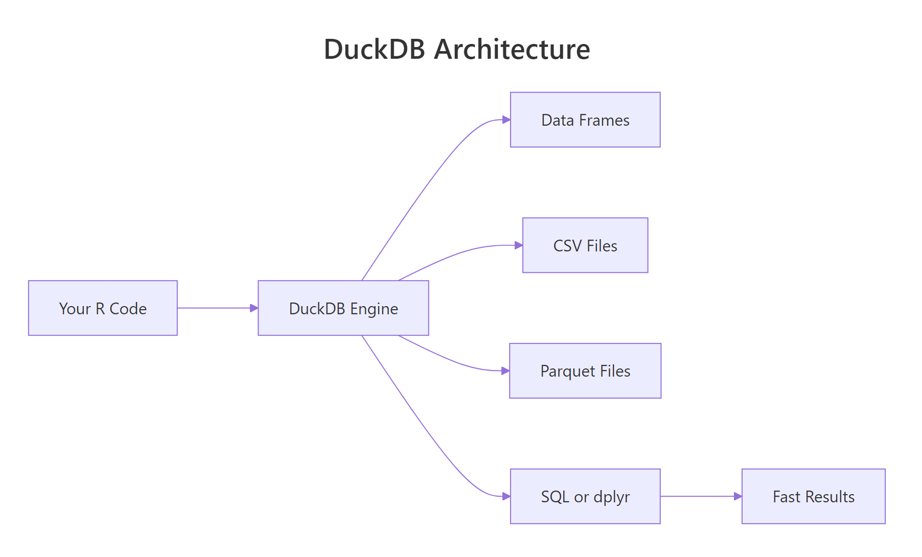
DuckDB architecture: in-process columnar engine

Figure 1: DuckDB runs inside the R process, no client-server round trips. Data lives in columnar format for vectorised queries.

Key Insight

"In-process" means DuckDB has no server. It is a library you load like ggplot2. There is nothing to install separately, nothing to configure, nothing to start. It just works.

Try it: Connect to DuckDB and run a trivial query.

RExercise: First DuckDB query

library(DBI); library(duckdb) con <- dbConnect(duckdb()) dbGetQuery(con, "SELECT 42 AS answer") dbDisconnect(con, shutdown = TRUE)

Click to reveal solution

RFirst DuckDB query solution

library(DBI); library(duckdb) con <- dbConnect(duckdb()) dbGetQuery(con, "SELECT 42 AS answer") #> answer #> 1 42 dbDisconnect(con, shutdown = TRUE)

This is the smallest possible DuckDB session, connect, run a single SELECT that needs no tables, disconnect. If this works, your installation is good.

How do you install DuckDB and run your first query?

Installation is one line:

RLoad DBI and duckdb

# install.packages("duckdb") library(DBI); library(duckdb)

Because DuckDB is C++ compiled into the R package, there is no separate binary to install, no environment variable, no driver to configure. The duckdb R package contains the entire database engine.

ROpen in-memory connection

con <- dbConnect(duckdb())

By default this gives you an in-memory database that vanishes when you disconnect. For persistent storage, pass a file path:

RPersistent and read-only connections

# Persistent database (creates the file if missing) con_disk <- dbConnect(duckdb(), dbdir = "my.duckdb") # Read-only access (faster for queries, safer for shared files) con_ro <- dbConnect(duckdb(), dbdir = "my.duckdb", read_only = TRUE)

From there, everything you already know from DBI works. Let's walk through a minimal workflow:

RQuery iris table with SQL

library(DBI); library(duckdb) con <- dbConnect(duckdb()) # 1. Load some data dbWriteTable(con, "iris_t", iris) # 2. Query with SQL dbGetQuery(con, " SELECT Species, AVG(\"Sepal.Length\") AS avg_len FROM iris_t GROUP BY Species ") #> Species avg_len #> 1 setosa 5.006 #> 2 versicolor 5.936 #> 3 virginica 6.588 dbDisconnect(con, shutdown = TRUE)

Three steps: connect, write, query. The column names from iris have dots in them, so SQL needs them in double quotes. Everything else is standard SQL.

Tip

Always pass shutdown = TRUE to dbDisconnect() for DuckDB. Without it, the in-process database keeps the file handle open, which can block subsequent connections. It is a harmless extra argument for SQLite-style databases but essential here.

Try it: Open an in-memory DuckDB, write mtcars, and query for the five cars with the highest mpg.

RExercise: Top five mpg cars

library(DBI); library(duckdb) con <- dbConnect(duckdb()) dbWriteTable(con, "cars", mtcars) # dbGetQuery(con, "SELECT * FROM cars ORDER BY mpg DESC LIMIT 5") dbDisconnect(con, shutdown = TRUE)

Click to reveal solution

RTop five mpg solution

dbGetQuery(con, "SELECT * FROM cars ORDER BY mpg DESC LIMIT 5") #> mpg cyl disp hp drat wt qsec vs am gear carb #> 1 33.9 4 71.1 65 4.22 1.835 19.90 1 1 4 1 #> 2 32.4 4 78.7 66 4.08 2.200 19.47 1 1 4 1 #> 3 30.4 4 75.7 52 4.93 1.615 18.52 1 1 4 2 #> 4 30.4 4 95.1113 3.77 1.513 16.90 1 1 5 2 #> 5 27.3 4 79.0 66 4.08 1.935 18.90 1 1 4 1

ORDER BY mpg DESC LIMIT 5 sorts the table descending and keeps only the top five rows, the standard SQL "top-N" pattern.

How do you query CSV and Parquet files without loading them?

This is where DuckDB really shines. You can point it at a file on disk and it queries the file directly, no read.csv, no temporary table, no RAM spike.

RQuery CSV and Parquet files

library(DBI); library(duckdb) con <- dbConnect(duckdb()) # Query a CSV file like it is a table # dbGetQuery(con, "SELECT * FROM 'large.csv' LIMIT 5") # Same idea for Parquet # dbGetQuery(con, "SELECT AVG(price) FROM 'sales.parquet'") # Filter and aggregate in one pass, reads only the columns/rows needed # dbGetQuery(con, " # SELECT region, SUM(revenue) # FROM 'sales.parquet' # WHERE year = 2025 # GROUP BY region # ") dbDisconnect(con, shutdown = TRUE)

Read "SELECT ... FROM 'file.csv'" as "treat this file as if it were a table in the database". DuckDB's CSV reader is battle-tested, it auto-detects separators, quotes, and types. For Parquet, the advantage is even bigger because the format is columnar on disk: if your query touches 3 out of 50 columns, DuckDB reads only those 3 from the file.

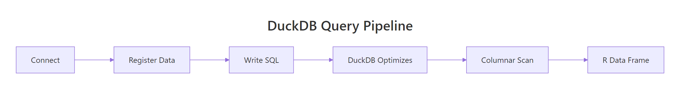
Query pipeline: file → parse → project → filter → aggregate

Figure 2: DuckDB's query pipeline. Projection (selecting columns) happens before the data is materialised, so wide files stay cheap to query.

For multiple files that share a schema, say, one CSV per day, use a glob pattern:

RUnion multiple Parquet files

# Read all 2025 Parquet files at once # dbGetQuery(con, "SELECT COUNT(*) FROM 'data/2025-*.parquet'")

The query planner treats the union of all matching files as one logical table. This is how DuckDB handles multi-file datasets without any manual concatenation.

Note

DuckDB's Parquet support includes predicate pushdown: WHERE year = 2025 is pushed into the Parquet reader, which skips entire row groups that can't match. On a 100-million-row file, you may scan only 5 million rows.

Try it: Write mtcars to a CSV and then query it directly from DuckDB without loading it first.

RExercise: Group mtcars CSV

library(DBI); library(duckdb) write.csv(mtcars, "mtcars_tmp.csv", row.names = FALSE) con <- dbConnect(duckdb()) # dbGetQuery(con, "SELECT cyl, AVG(mpg) FROM 'mtcars_tmp.csv' GROUP BY cyl") dbDisconnect(con, shutdown = TRUE)

Click to reveal solution

RGroup mtcars CSV solution

dbGetQuery(con, "SELECT cyl, AVG(mpg) AS avg_mpg FROM 'mtcars_tmp.csv' GROUP BY cyl ORDER BY cyl") #> cyl avg_mpg #> 1 4 26.66364 #> 2 6 19.74286 #> 3 8 15.10000

DuckDB treats 'mtcars_tmp.csv' as if it were a table name. The CSV reader auto-detects the schema and only reads the columns the query needs, no read.csv step required.

How does DuckDB compare to SQLite and data.table?

All three are fast, but they target different problems.

Feature	SQLite	DuckDB	data.table
In-process	Yes	Yes	Yes
Query language	SQL	SQL + dplyr	`[i, j, by]`
Storage format	Row-based	Columnar	In-memory only
Multi-threaded	No	Yes	Yes
Query larger than RAM	Limited	Yes	No
Direct CSV/Parquet query	No	Yes	No

SQLite is optimized for transactional workloads, small, frequent reads and writes on a single row at a time. It is the right choice for configuration files, offline apps, and small datasets. It is not optimised for "aggregate over 10 million rows".

data.table is the fastest in-memory table library in R. It is perfect for datasets that fit in RAM and when you want R syntax, not SQL. But it cannot query Parquet files and does not stream larger-than-RAM data.

DuckDB fills the sweet spot between the two: analytical speed on datasets that might or might not fit in memory, with a query language (SQL) that is widely understood and already known by anyone with a data warehouse background.

RRegister data frame zero-copy

library(DBI); library(duckdb) # DuckDB can register an R data frame as a zero-copy view con <- dbConnect(duckdb()) duckdb_register(con, "mt", mtcars) # Query it without copying anything dbGetQuery(con, "SELECT cyl, COUNT(*) FROM mt GROUP BY cyl") #> cyl COUNT(*) #> 1 6 7 #> 2 4 11 #> 3 8 14 dbDisconnect(con, shutdown = TRUE)

duckdb_register() is a clever trick: DuckDB reads directly from your R data frame's memory, so there is zero copy, zero serialization, and zero additional RAM usage. For quick joins between a big Parquet file and a small R reference table, it is the ideal pattern.

Tip

If your data fits in RAM and you love R syntax, use data.table. If it fits in RAM but you prefer SQL or dplyr, use DuckDB. If it does not fit in RAM, use DuckDB. If you need transactional writes from multiple processes, use SQLite or PostgreSQL.

Try it: Register iris as a DuckDB view using duckdb_register() and run a GROUP BY query on it.

RExercise: Register iris view

library(DBI); library(duckdb) con <- dbConnect(duckdb()) duckdb_register(con, "iris_v", iris) # dbGetQuery(con, "SELECT Species, COUNT(*) FROM iris_v GROUP BY Species") dbDisconnect(con, shutdown = TRUE)

Click to reveal solution

RRegister iris view solution

dbGetQuery(con, "SELECT Species, COUNT(*) AS n FROM iris_v GROUP BY Species ORDER BY Species") #> Species n #> 1 setosa 50 #> 2 versicolor 50 #> 3 virginica 50

duckdb_register() exposes the R data frame as a virtual table without copying it. From DuckDB's point of view it looks just like any other table you can query, group, and join.

How do you use DuckDB with dplyr via dbplyr or duckplyr?

Two options. The older path is dbplyr via DBI, exactly like any other database. The newer path is duckplyr, a drop-in replacement for dplyr that is powered by DuckDB under the hood.

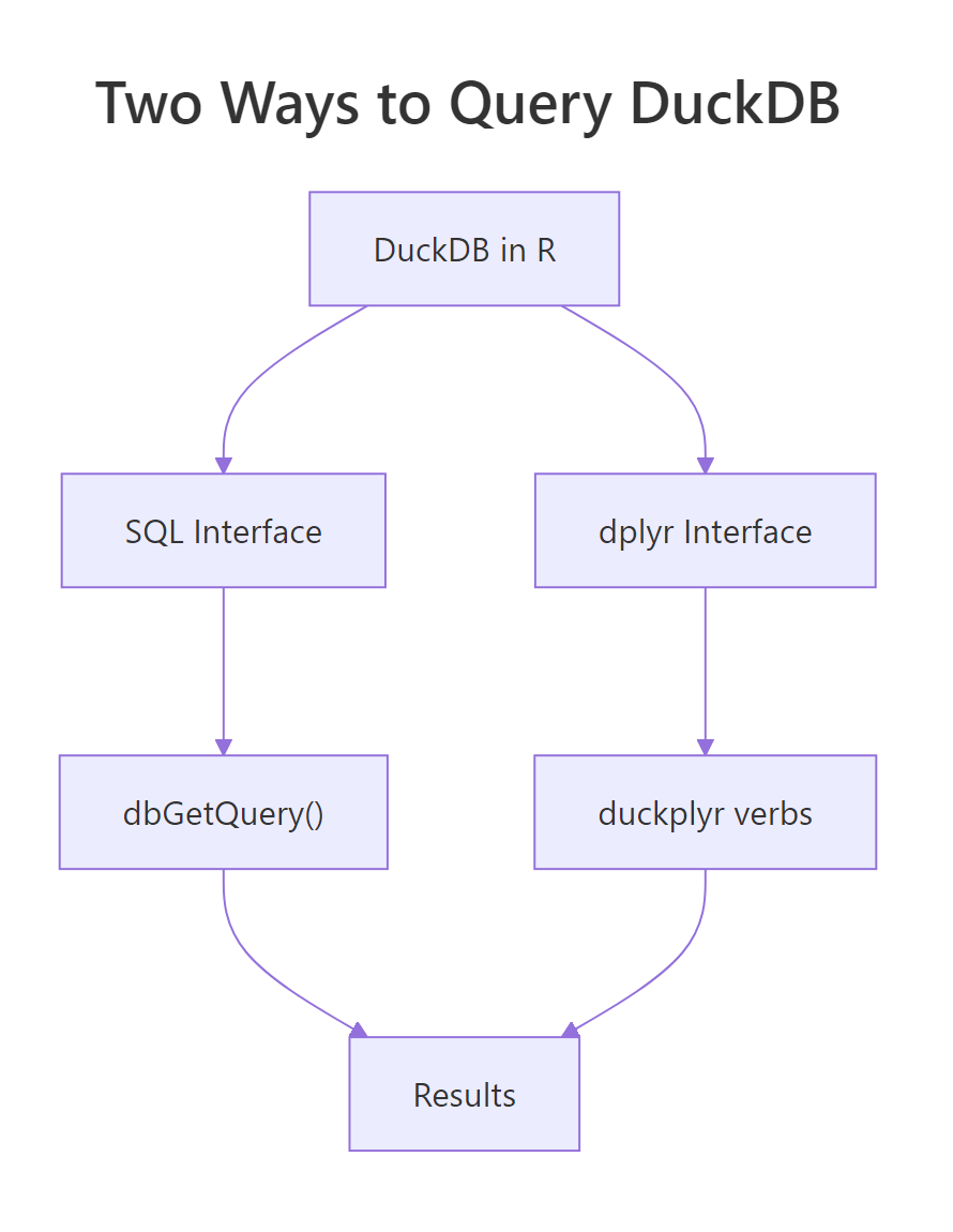
Two interfaces: SQL via DBI vs dplyr via duckplyr

Figure 3: Two ways to talk to DuckDB from R. Pick the one that matches your team's background.

Rdbplyr pipeline over DuckDB

library(DBI); library(duckdb); library(dplyr); library(dbplyr) con <- dbConnect(duckdb()) duckdb_register(con, "mt", mtcars) tbl(con, "mt") |> filter(mpg > 20) |> group_by(cyl) |> summarise(avg_hp = mean(hp)) |> arrange(desc(avg_hp)) |> collect() #> # A tibble: 3 x 2 #> cyl avg_hp #> <dbl> <dbl> #> 1 6 110 #> 2 4 78.5 #> 3 8 NaN

Same dplyr you write every day. The collect() at the end runs the generated SQL and brings the result back as a tibble. show_query() lets you see the SQL if you want to learn or debug.

The newer duckplyr package goes one step further: you do not even see the DBI calls.

Rduckplyr drop-in replacement

# library(duckplyr) # mtcars |> # as_duckplyr_df() |> # filter(mpg > 20) |> # group_by(cyl) |> # summarise(avg_hp = mean(hp))

Syntactically identical to dplyr. Behind the scenes, duckplyr turns each verb into DuckDB execution, so the whole pipeline runs at the native speed of the engine, often 5-50x faster than plain dplyr for group-and-aggregate workloads.

Warning

duckplyr matches dplyr's API but not every function is supported yet. If a verb falls through, the pipeline may quietly execute in base dplyr, losing the speedup. Check the duckplyr documentation for coverage before betting a production job on it.

Try it: Use dbplyr to filter and summarize a DuckDB-registered iris.

RExercise: dbplyr filter irisv

library(DBI); library(duckdb); library(dplyr); library(dbplyr) con <- dbConnect(duckdb()) duckdb_register(con, "iris_v", iris) # tbl(con, "iris_v") |> filter(Petal.Length > 4) |> group_by(Species) |> summarise(n = n()) |> collect() dbDisconnect(con, shutdown = TRUE)

Click to reveal solution

Rdbplyr irisv solution

tbl(con, "iris_v") |> filter(Petal.Length > 4) |> group_by(Species) |> summarise(n = n()) |> collect() #> # A tibble: 2 x 2 #> Species n #> <fct> <int> #> 1 versicolor 34 #> 2 virginica 50

The dplyr verbs are translated to SQL by dbplyr and executed inside DuckDB. setosa drops out because all of its petals are shorter than 4 cm, so the group has no rows after the filter.

When should you persist a DuckDB file vs use in-memory?

In-memory mode (dbConnect(duckdb()) with no path) is perfect when:

You are querying a CSV or Parquet file directly, the DuckDB "database" is just a scratch space for the query planner.
Your workflow is stateless, every script run starts fresh.
You want maximum speed, no disk I/O for intermediate state.

Persistent mode (dbConnect(duckdb(), dbdir = "file.duckdb")) is the right choice when:

You are building a derived dataset that will be re-used across scripts or sessions.
You have intermediate tables from ETL jobs that are expensive to re-compute.
Multiple processes need to share the same tables (though only one can write at a time).

RMaterialise table with CTAS

library(DBI); library(duckdb) # Build-once, query-many pattern con <- dbConnect(duckdb(), dbdir = "analytics.duckdb") # Materialize an expensive query once dbExecute(con, " CREATE OR REPLACE TABLE monthly_sales AS SELECT strftime(order_date, '%Y-%m') AS month, SUM(amount) AS revenue FROM read_csv_auto('raw/orders_*.csv') GROUP BY 1 ") # Later sessions query the materialised table cheaply # dbGetQuery(con, "SELECT * FROM monthly_sales ORDER BY month") dbDisconnect(con, shutdown = TRUE)

The CREATE OR REPLACE TABLE ... AS SELECT pattern (CTAS) materializes the result of a query into a named table. For ETL and reporting workflows, this is the bread-and-butter idiom.

Note

A DuckDB file is a single .duckdb file on disk, easy to back up, version, or share. Unlike PostgreSQL, there is no cluster directory or permissions to worry about.

Try it: Create a persistent DuckDB file, write a table, disconnect, reconnect, and verify the table is still there.

RExercise: Round-trip persistent table

library(DBI); library(duckdb) con <- dbConnect(duckdb(), dbdir = "tmp.duckdb") dbWriteTable(con, "t", data.frame(x = 1:5)) dbDisconnect(con, shutdown = TRUE) con2 <- dbConnect(duckdb(), dbdir = "tmp.duckdb") # dbReadTable(con2, "t") dbDisconnect(con2, shutdown = TRUE)

Click to reveal solution

RPersistent table round-trip solution

con2 <- dbConnect(duckdb(), dbdir = "tmp.duckdb") dbReadTable(con2, "t") #> x #> 1 1 #> 2 2 #> 3 3 #> 4 4 #> 5 5 dbDisconnect(con2, shutdown = TRUE)

Because the first connection wrote to a file (dbdir = "tmp.duckdb") instead of memory, the table survives the disconnect. Reconnecting to the same file path gives a new session that sees all previously stored tables.

How do you handle larger-than-memory data with DuckDB?

DuckDB's secret weapon is that it can spill to disk when a query's intermediate state exceeds RAM. Joins, sorts, and large GROUP BY operations all spill automatically. You do not have to configure anything.

RQuery 50GB Parquet on laptop

# Imagine 'big.parquet' is 50 GB; your laptop has 16 GB RAM library(DBI); library(duckdb) con <- dbConnect(duckdb()) # result <- dbGetQuery(con, " # SELECT customer_id, SUM(amount) AS total # FROM 'big.parquet' # WHERE year = 2025 # GROUP BY customer_id # ORDER BY total DESC # LIMIT 100 # ") dbDisconnect(con, shutdown = TRUE)

The aggregate is computed in streaming fashion, DuckDB reads the Parquet file one row group at a time, maintains a partial hash table per customer, and spills to a temporary file when memory pressure gets high. You get a 100-row result from a 50-GB input.

Three tips for very large data:

Use Parquet, not CSV. Parquet is compressed and columnar, often 10x smaller on disk and much faster to query.
Filter early. Put WHERE clauses on columns that exist in the file, so DuckDB can skip entire row groups via predicate pushdown.
Limit memory with memory_limit if needed. dbExecute(con, "SET memory_limit = '4GB'") caps DuckDB to 4 GB and forces aggressive spilling.

RSet memorylimit and threads

# Set a memory limit for a big ETL job library(DBI); library(duckdb) con <- dbConnect(duckdb()) dbExecute(con, "SET memory_limit = '4GB'") dbExecute(con, "SET threads = 4") # Run your huge query here dbDisconnect(con, shutdown = TRUE)

SET threads = 4 tells DuckDB to use 4 parallel threads, on a laptop with 8 cores, 4 is often a good balance between query speed and leaving cores for the rest of your workflow.

Key Insight

With DuckDB, "bigger than RAM" is no longer a special case, it is just a normal query that takes a bit longer. For most R users, this one feature alone justifies the switch from pandas-style pipelines.

Try it: Use SET memory_limit to cap DuckDB at 2 GB and SET threads to 2.

RExercise: Configure DuckDB limits

library(DBI); library(duckdb) con <- dbConnect(duckdb()) dbExecute(con, "SET memory_limit = '2GB'") dbExecute(con, "SET threads = 2") dbDisconnect(con, shutdown = TRUE)

Click to reveal solution

RConfigure DuckDB limits solution

library(DBI); library(duckdb) con <- dbConnect(duckdb()) dbExecute(con, "SET memory_limit = '2GB'") #> [1] 0 dbExecute(con, "SET threads = 2") #> [1] 0 # Verify the settings took effect dbGetQuery(con, "SELECT current_setting('memory_limit') AS memory_limit, current_setting('threads') AS threads") #> memory_limit threads #> 1 1.9 GiB 2 dbDisconnect(con, shutdown = TRUE)

SET memory_limit and SET threads are session-level pragmas, they apply to the current connection. The [1] 0 from dbExecute() is the affected-row count (zero, because no data rows changed).

Practice Exercises

Exercise 1: Register and query

Solution

RPractice: Average mpg per cyl

library(DBI); library(duckdb) con <- dbConnect(duckdb()) duckdb_register(con, "mt", mtcars) dbGetQuery(con, "SELECT cyl, AVG(mpg) AS avg_mpg FROM mt GROUP BY cyl ORDER BY cyl") dbDisconnect(con, shutdown = TRUE)

Exercise 2: Query a CSV directly

Write iris to a CSV file and query it with DuckDB without loading it into R first.

Solution

RPractice: Group iris CSV

library(DBI); library(duckdb) write.csv(iris, "iris_tmp.csv", row.names = FALSE) con <- dbConnect(duckdb()) dbGetQuery(con, "SELECT Species, COUNT(*) AS n FROM 'iris_tmp.csv' GROUP BY Species") dbDisconnect(con, shutdown = TRUE)

Exercise 3: CTAS and reuse

Create a persistent DuckDB file with a materialised table of average petal length per species, then reconnect and read it.

Solution

RPractice: Persist avgpetal table

library(DBI); library(duckdb) con <- dbConnect(duckdb(), dbdir = "iris.duckdb") duckdb_register(con, "iris_v", iris) dbExecute(con, "CREATE OR REPLACE TABLE avg_petal AS SELECT Species, AVG(\"Petal.Length\") AS avg_pl FROM iris_v GROUP BY Species") dbDisconnect(con, shutdown = TRUE) con2 <- dbConnect(duckdb(), dbdir = "iris.duckdb") dbReadTable(con2, "avg_petal") dbDisconnect(con2, shutdown = TRUE)

Complete Example

End-to-end analytics workflow: load data, query with both SQL and dplyr, materialise the result.

REnd-to-end sales analytics pipeline

library(DBI); library(duckdb); library(dplyr); library(dbplyr); library(tibble) con <- dbConnect(duckdb()) on.exit(dbDisconnect(con, shutdown = TRUE)) # Step 1: create sample sales data sales <- tibble( order_id = 1:200, customer = sample(c("Asha","Bilal","Cleo","Daan","Edu"), 200, replace = TRUE), region = sample(c("N","S","E","W"), 200, replace = TRUE), amount = round(runif(200, 10, 500), 2), month = sample(1:12, 200, replace = TRUE) ) duckdb_register(con, "sales", sales) # Step 2: SQL version dbGetQuery(con, " SELECT region, month, SUM(amount) AS revenue FROM sales GROUP BY region, month ORDER BY region, month LIMIT 10 ") # Step 3: equivalent dplyr version tbl(con, "sales") |> group_by(region, month) |> summarise(revenue = sum(amount, na.rm = TRUE), .groups = "drop") |> arrange(region, month) |> head(10) |> collect() # Step 4: materialise the top customers for reuse dbExecute(con, " CREATE OR REPLACE TABLE top_customers AS SELECT customer, SUM(amount) AS revenue FROM sales GROUP BY customer ORDER BY revenue DESC LIMIT 5 ") dbReadTable(con, "top_customers")

Two interfaces, one engine, identical results. Use SQL when you are collaborating with data engineers, dplyr when you are deep in a tidyverse pipeline. The runtime is the same because DuckDB does the work in both cases.

Summary

Task	Function / SQL
Connect in-memory	`dbConnect(duckdb())`
Connect persistent	`dbConnect(duckdb(), dbdir = "file.duckdb")`
Zero-copy register df	`duckdb_register(con, "name", df)`
Query CSV directly	`SELECT * FROM 'file.csv'`
Query Parquet directly	`SELECT * FROM 'file.parquet'`
Multi-file glob	`SELECT * FROM 'data/2025-*.parquet'`
Materialise a result	`CREATE OR REPLACE TABLE x AS SELECT ...`
Cap memory	`SET memory_limit = '4GB'`
Set thread count	`SET threads = 4`
Always disconnect with	`dbDisconnect(con, shutdown = TRUE)`

Four rules:

Use DuckDB for analytics, SQLite for transactions. Different tools for different jobs.
Register, don't copy. duckdb_register() makes a data frame queryable with zero overhead.
Query files directly. Skip the read.csv/read_parquet step entirely.
Always shutdown = TRUE. It prevents dangling file handles on disconnect.

References

Continue Learning

DBI in R, the interface DuckDB uses; learn DBI once, use it with any database.
dplyr group_by() and summarise(), translate directly to DuckDB via dbplyr.
Importing Data in R, DuckDB complements the traditional read_csv/read_parquet workflow.

{% endraw %}

DuckDB in R: Query 100 Million Rows on Your Laptop in Under 2 Seconds

Why is DuckDB faster than reading a CSV?

How do you install DuckDB and run your first query?

How do you query CSV and Parquet files without loading them?

How does DuckDB compare to SQLite and data.table?

How do you use DuckDB with dplyr via dbplyr or duckplyr?

When should you persist a DuckDB file vs use in-memory?

How do you handle larger-than-memory data with DuckDB?

Practice Exercises

Exercise 1: Register and query

Exercise 2: Query a CSV directly

Exercise 3: CTAS and reuse

Complete Example

Summary

References

Continue Learning

Further Reading

Related Tutorials