patchwork in R: Combine Multiple ggplot2 Plots With Aligned Axes and Shared Legends

The patchwork package makes it ridiculously simple to combine multiple ggplot2 plots into a single figure, just add them together with +, stack them with /, or place them side-by-side with |, and patchwork handles alignment, spacing, and shared legends automatically.

How do you combine two ggplot2 plots with patchwork?

Combining plots is one of the most common tasks in data visualization. Maybe you've built a scatter plot and a histogram that tell a richer story side by side, or you need a multi-panel figure for a report. patchwork lets you do this in one line of code, literally add two plots together.

RInteractive R

library(ggplot2) library(patchwork) p1 <- ggplot(mtcars, aes(wt, mpg)) + geom_point(color = "steelblue", size = 2) + labs(title = "Weight vs MPG") p2 <- ggplot(mtcars, aes(mpg)) + geom_histogram(fill = "coral", bins = 10) + labs(title = "MPG Distribution") p1 + p2 #> [A composite figure: scatter plot on the left, histogram on the right]

That + operator is doing all the work. patchwork overloads + so that when you "add" two ggplot objects, it places them side by side in a grid. No grid.arrange(), no complicated layout matrices, just +.

But + isn't your only option. patchwork gives you two more operators that communicate your intent more clearly.

RInteractive R

# Horizontal: same as + but explicit p1 | p2 #> [Two plots placed side by side] # Vertical: stack on top of each other p1 / p2 #> [Scatter plot on top, histogram below]

The | operator forces horizontal placement and / forces vertical stacking. Use | and / when you want to be explicit about direction, they make your layout code read like a description of the figure.

Tip

patchwork only works with ggplot2 objects. Base R plots created with plot() or hist() won't work directly. Wrap them in wrap_elements(~plot(...)) if you need to mix base and ggplot2 graphics.

Try it: Create a boxplot of mpg by cyl and a bar chart counting cars per gear from the mtcars dataset, then combine them horizontally with |.

RInteractive R

# Try it: combine a boxplot and bar chart ex_box <- ggplot(mtcars, aes(factor(cyl), mpg)) + geom_boxplot() ex_bar <- ggplot(mtcars, aes(factor(gear))) + geom_bar() # Combine horizontally: # your code here

Click to reveal solution

RInteractive R

ex_box <- ggplot(mtcars, aes(factor(cyl), mpg)) + geom_boxplot(fill = "lightblue") + labs(x = "Cylinders", y = "MPG") ex_bar <- ggplot(mtcars, aes(factor(gear))) + geom_bar(fill = "salmon") + labs(x = "Gears", y = "Count") ex_box | ex_bar #> [Boxplot on the left, bar chart on the right]

Explanation: The | operator explicitly places the two plots side by side, just like + would, but communicates horizontal intent more clearly.

How do you control the number of rows and columns?

When you combine more than two plots, patchwork arranges them in an auto-calculated grid, trying to keep things roughly square. But often you want a specific layout, like everything in one column or a 2×3 grid.

The plot_layout() function gives you that control. Think of it as the layout manager: it tells patchwork how many rows and columns to use.

RInteractive R

p3 <- ggplot(mtcars, aes(hp, qsec)) + geom_point(color = "forestgreen", size = 2) + labs(title = "HP vs Quarter Mile") # Default: patchwork auto-arranges (here: 1 row, 3 cols) p1 + p2 + p3 # Force a single column: p1 + p2 + p3 + plot_layout(ncol = 1) #> [Three plots stacked vertically in one column]

The ncol = 1 argument forces all three plots into a single column. You could also use nrow = 1 to force a single row, or specify both for exact control.

What if your plots shouldn't all be the same size? The widths and heights arguments let you set relative proportions.

RInteractive R

# Make the scatter plot twice as wide as the histogram p1 + p2 + plot_layout(widths = c(2, 1)) #> [Scatter plot takes 2/3 of the width, histogram takes 1/3]

Key Insight

widths and heights are relative ratios, not pixel values. Setting widths = c(2, 1) means the first plot gets twice the space of the second. The values c(2, 1), c(4, 2), and c(200, 100) all produce the same layout.

Try it: Arrange four plots (p1, p2, p3, and a new density plot) in a 2×2 grid where the left column is three times wider than the right.

RInteractive R

# Try it: 2x2 grid with custom widths ex_dens <- ggplot(mtcars, aes(hp)) + geom_density(fill = "plum") # Arrange in 2x2 with widths c(3, 1): # your code here

Click to reveal solution

RInteractive R

ex_dens <- ggplot(mtcars, aes(hp)) + geom_density(fill = "plum") + labs(title = "HP Density") p1 + p2 + p3 + ex_dens + plot_layout(ncol = 2, widths = c(3, 1)) #> [2x2 grid: left column 3x wider than right]

Explanation: ncol = 2 creates two columns, and widths = c(3, 1) makes the left column occupy 75% of the width.

How do you build complex layouts with nesting and design strings?

Real figures often need more than a uniform grid. You might want two small plots on top and one wide plot spanning the bottom. Patchwork gives you two ways to build these complex arrangements: nesting with parentheses and design strings.

Parentheses create sub-layouts within your composition. Everything inside parentheses gets arranged as a group first, then that group takes up one slot in the outer layout.

RInteractive R

# Two plots on top, one wide plot spanning the full bottom (p1 | p2) / p3 #> [Row 1: scatter + histogram side by side. Row 2: HP plot spanning full width]

That reads almost like a sentence: "p1 beside p2, above p3." The parentheses group the top row, and / stacks it above p3.

For even more control, design strings let you sketch out your layout using a text grid. Each letter represents one plot, and # marks empty cells.

RInteractive R

design <- " AAB ACC " p1 + p2 + p3 + plot_layout(design = design) #> [Plot A (p1) spans top-left and bottom-left. Plot B (p2) is top-right. #> Plot C (p3) is bottom-right.]

Each letter in the design string maps to a plot in the order they were added. Plot A (p1) fills four cells, Plot B (p2) gets one cell top-right, and Plot C (p3) gets one cell bottom-right. This is the most flexible layout approach patchwork offers.

Tip

Use # in design strings for empty cells. For example, "A#\n#B" puts plot A top-left and plot B bottom-right with empty space in between.

Try it: Create a layout where one wide plot spans the entire top row and two plots sit below it, side by side. Use either nesting with parentheses or a design string.

RInteractive R

# Try it: one plot on top, two below # Hint: try p3 / (p1 | p2) or a design string # your code here

Click to reveal solution

RInteractive R

# Using nesting: p3 / (p1 | p2) #> [HP plot spans full width on top. Scatter + histogram side by side below.]

Explanation: (p1 | p2) groups the bottom row horizontally, then / stacks p3 above it.

How do you share legends and collect axes across plots?

When multiple plots use the same color mapping, you end up with duplicate legends, one per plot. That wastes space and looks cluttered. patchwork's guides = "collect" gathers identical legends into one.

Let's build three scatter plots that all color points by the number of cylinders.

RInteractive R

p_scatter1 <- ggplot(mtcars, aes(wt, mpg, color = factor(cyl))) + geom_point(size = 2) + labs(title = "Weight vs MPG") p_scatter2 <- ggplot(mtcars, aes(hp, mpg, color = factor(cyl))) + geom_point(size = 2) + labs(title = "HP vs MPG") p_scatter3 <- ggplot(mtcars, aes(disp, mpg, color = factor(cyl))) + geom_point(size = 2) + labs(title = "Displacement vs MPG") p_scatter1 + p_scatter2 + p_scatter3 + plot_layout(guides = "collect") #> [Three scatter plots side by side with ONE shared legend on the right]

Instead of three identical legends eating up space, patchwork detects that all three use the same color mapping and keeps just one copy. The legend moves to the position defined by the global theme (right side by default).

Shared axes work similarly. When side-by-side plots share the same y-axis, displaying it on every panel is redundant. The axes argument handles this.

RInteractive R

pa <- ggplot(mtcars, aes(wt, mpg)) + geom_point() + labs(title = "Weight") pb <- ggplot(mtcars, aes(hp, mpg)) + geom_point() + labs(title = "Horsepower") pa + pb + plot_layout(axes = "collect") #> [Two scatter plots: only the left one shows y-axis labels]

With axes = "collect", the redundant y-axis on the right plot disappears. If you only want to merge the axis titles (but keep the tick labels), use axis_titles = "collect" instead.

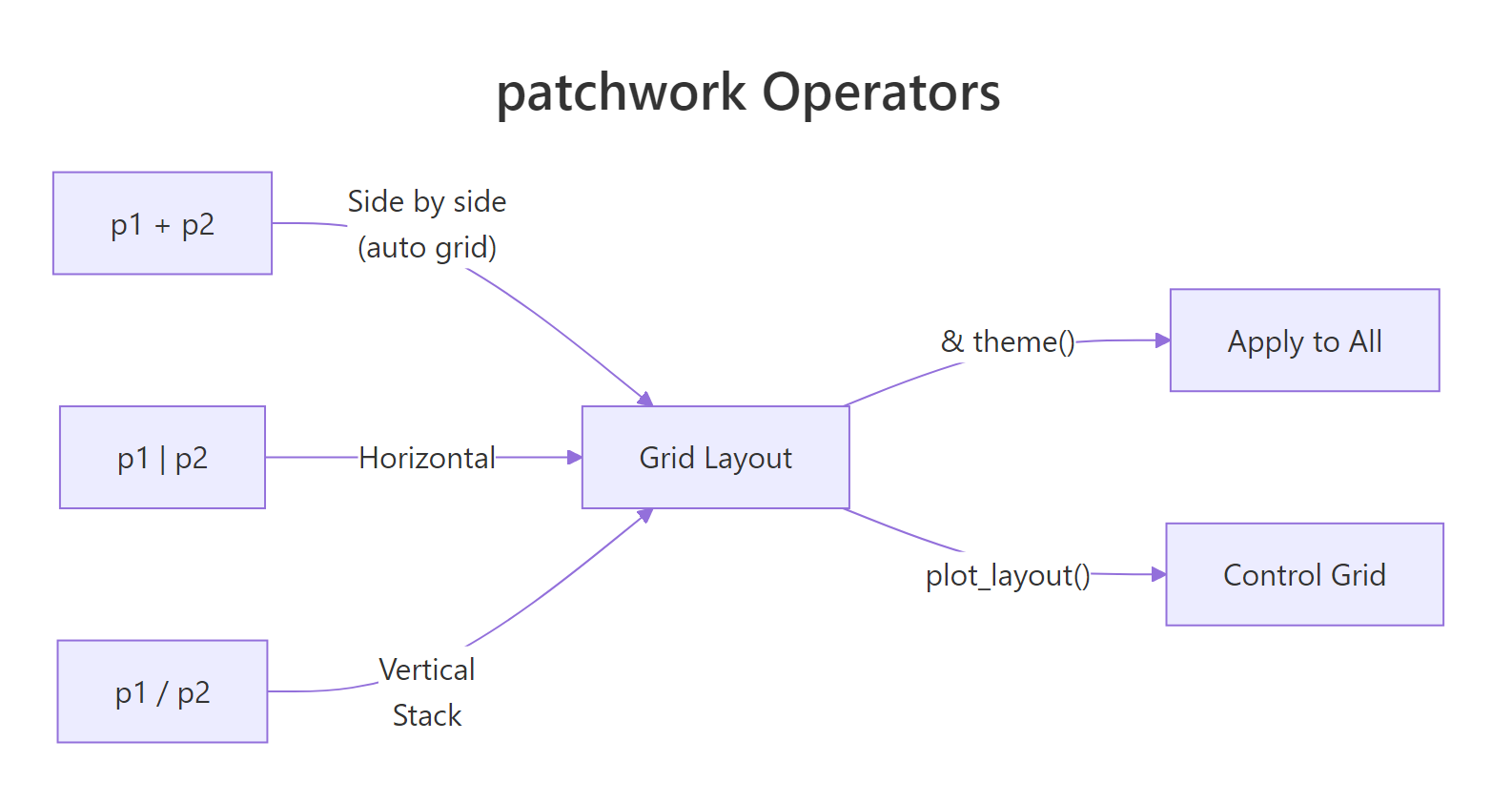
How patchwork operators combine plots into layouts

Figure 1: How patchwork operators combine plots into layouts.

Key Insight

Guides are matched by visual appearance, not variable name. If two plots use color = factor(cyl) with the same scale, patchwork recognizes them as duplicates. But if one uses a custom color palette and the other doesn't, patchwork treats them as different legends.

Try it: Create two scatter plots from mtcars, one mapping wt to x and one mapping hp to x, both coloring by factor(cyl). Combine them and collect the shared legend.

RInteractive R

# Try it: collect shared legends ex_s1 <- ggplot(mtcars, aes(wt, mpg, color = factor(cyl))) + geom_point() ex_s2 <- ggplot(mtcars, aes(hp, mpg, color = factor(cyl))) + geom_point() # Combine with shared legend: # your code here

Click to reveal solution

RInteractive R

ex_s1 <- ggplot(mtcars, aes(wt, mpg, color = factor(cyl))) + geom_point(size = 2) + labs(color = "Cylinders") ex_s2 <- ggplot(mtcars, aes(hp, mpg, color = factor(cyl))) + geom_point(size = 2) + labs(color = "Cylinders") ex_s1 + ex_s2 + plot_layout(guides = "collect") #> [Two scatter plots with a single shared color legend]

Explanation: Both plots use the same color aesthetic and scale, so guides = "collect" merges them into one legend positioned on the right.

How do you add titles, subtitles, and panel tags?

Publication-quality figures need more than just the individual plot titles, they need an overall title that describes the entire composition and panel labels like (A), (B), (C) so you can reference specific panels in your text.

plot_annotation() handles both. It adds metadata that sits above or below the entire combined figure.

RInteractive R

(p1 | p2 | p3) + plot_annotation( title = "Motor Trends Car Analysis", subtitle = "Three views of the mtcars dataset", caption = "Source: 1974 Motor Trend US magazine", tag_levels = "A" ) #> [Three plots labeled (A), (B), (C) with an overall title and subtitle]

The tag_levels = "A" argument auto-labels each panel as A, B, C. Other options include "1" for numbers, "i" for lowercase Roman numerals, and "I" for uppercase Roman numerals.

You can customize how tags look by modifying the plot.tag theme element. The & operator (which we'll cover in the next section) applies the theme change to every panel.

RInteractive R

(p1 | p2 | p3) + plot_annotation(tag_levels = "A") & theme(plot.tag = element_text(size = 14, face = "bold")) #> [Three plots with bold, larger panel tags A, B, C]

Note

Tag levels can be nested for sub-panels. Use tag_levels = c("A", "1") to get A1, A2, B1, B2 when you have nested patchworks. This is useful for complex multi-panel figures in academic publications.

Try it: Create a 3-panel figure using p1, p2, and p3, add panel tags using Roman numerals ("I"), and give the figure an overall title.

RInteractive R

# Try it: annotated figure with Roman numeral tags # your code here

Click to reveal solution

RInteractive R

(p1 | p2 | p3) + plot_annotation( title = "mtcars Overview", tag_levels = "I" ) #> [Three plots labeled (I), (II), (III) with overall title]

Explanation: tag_levels = "I" produces uppercase Roman numerals. plot_annotation() places the title above all three panels.

How do you modify all plots at once with & and *?

After combining plots, you often want to apply the same theme or modification to every panel, switching all plots to theme_minimal(), for instance, or changing font sizes across the board. patchwork's & operator does exactly this.

RInteractive R

(p1 | p2 | p3) & theme_minimal() #> [All three plots now use theme_minimal(), clean, gridline-only backgrounds]

The & operator reaches into every plot in the composition and applies whatever modification you put after it. It's the "broadcast" operator, one change, applied everywhere.

But what if you have nested layouts and only want to modify the outer level? That's where * comes in. It applies modifications only to the current nesting level, without reaching into nested sub-patchworks.

RInteractive R

# & reaches into nested patchwork nested <- (p1 | p2) / p3 nested & theme_bw() #> [All three plots use theme_bw()] # * only affects the current level nested * theme_bw() #> [Only the top-level arrangement is affected, p1 and p2 keep their original theme if nested deeper]

In practice, & is what you'll use 95% of the time. The * operator matters when you build deeply nested compositions where inner sub-layouts should keep their own styling.

Warning

& reaches into nested patchworks but * does not. If you're seeing unexpected theme behavior, check whether you're using & (broadcast to all) or * (current level only). This distinction only matters with nested layouts.

Try it: Combine p1, p2, and p3 and apply & theme_bw() to change all their themes at once.

RInteractive R

# Try it: apply theme to all plots at once # your code here

Click to reveal solution

RInteractive R

(p1 | p2 | p3) & theme_bw() #> [All three plots now use theme_bw(), white background with border]

Explanation: The & operator broadcasts theme_bw() to every plot in the patchwork, overriding their default theme.

How do you add insets and spacers?

Sometimes you need a small plot overlaid on a larger one, like a zoomed-in detail view, a summary statistic, or a mini-map. patchwork's inset_element() places one plot on top of another without consuming a grid cell.

Let's overlay a zoomed scatter plot on top of the full view.

RInteractive R

p_full <- ggplot(mtcars, aes(wt, mpg)) + geom_point(color = "steelblue", size = 2) + labs(title = "Full View: Weight vs MPG") p_inset <- ggplot(mtcars[mtcars$wt < 3, ], aes(wt, mpg)) + geom_point(color = "red", size = 2) + labs(title = "Zoomed: wt < 3") + theme_minimal(base_size = 8) p_full + inset_element(p_inset, left = 0.55, bottom = 0.55, right = 0.99, top = 0.99) #> [Full scatter plot with a small zoomed-in version in the top-right corner]

The left, bottom, right, and top arguments position the inset using 0-1 coordinates relative to the panel area. So left = 0.55, bottom = 0.55 puts the inset's lower-left corner just past the middle of both axes.

For adding empty space between plots, maybe for visual breathing room or to align with a non-plot element, use plot_spacer().

RInteractive R

p1 + plot_spacer() + p2 #> [Scatter plot, empty space, histogram, three equally-sized columns]

The spacer takes up one cell in the grid, creating a gap between your plots.

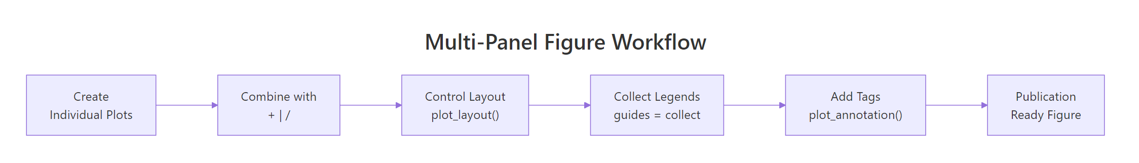
The multi-panel figure workflow from individual plots to publication-ready output

Figure 2: The multi-panel figure workflow from individual plots to publication-ready output.

Tip

inset_element() positions use 0-1 coordinates relative to the panel area. Set align_to = "plot" to position relative to the full plot area (including margins), or align_to = "full" for the entire figure.

Try it: Place a plot_spacer() between p1 and p2 in a horizontal layout, creating a visual gap.

RInteractive R

# Try it: add a spacer between two plots # your code here

Click to reveal solution

RInteractive R

p1 + plot_spacer() + p2 #> [Scatter plot | empty space | histogram]

Explanation: plot_spacer() creates an empty cell in the grid layout, producing visible separation between the two plots.

Practice Exercises

Exercise 1: Multi-panel iris figure with shared legend

Build a 3-panel publication figure from the iris dataset:

Panel A: scatter plot of Sepal.Length vs Sepal.Width, colored by Species
Panel B: boxplot of Petal.Length by Species, colored by Species
Panel C: histogram of Petal.Width, filled by Species

Use a design string to place A on the left spanning both rows, B top-right, and C bottom-right. Collect the shared legend, add panel tags (A/B/C), and give the figure an overall title "Iris Dataset Overview."

RInteractive R

# Exercise 1: multi-panel iris figure # Hint: design = "AB\nAC", then plot_layout(design=..., guides="collect") # Write your code below:

Click to reveal solution

RInteractive R

my_scatter <- ggplot(iris, aes(Sepal.Length, Sepal.Width, color = Species)) + geom_point(size = 2) + labs(title = "Sepal Dimensions") my_box <- ggplot(iris, aes(Species, Petal.Length, fill = Species)) + geom_boxplot() + labs(title = "Petal Length") my_hist <- ggplot(iris, aes(Petal.Width, fill = Species)) + geom_histogram(bins = 15, alpha = 0.7, position = "identity") + labs(title = "Petal Width") my_design <- "AB AC" my_scatter + my_box + my_hist + plot_layout(design = my_design, guides = "collect") + plot_annotation( title = "Iris Dataset Overview", tag_levels = "A" ) #> [Three-panel figure: scatter spanning left column, boxplot top-right, #> histogram bottom-right. Single shared legend. Tags A, B, C.]

Explanation: The design string "AB\nAC" allocates two rows and two columns: plot A fills the entire left column (rows 1 and 2), while B and C each get one cell on the right. guides = "collect" merges the Species legends.

Exercise 2: Diamond dashboard with inset

Create a 4-panel dashboard from the diamonds dataset (use a 5000-row sample for speed):

Price distribution histogram
Carat vs price scatter plot (colored by cut)
Bar chart of diamond cuts
An inset with a small density plot of log(price) overlaid on the histogram panel

Arrange panels 1-3 in a custom layout. Use & theme_minimal(), collect guides, and add an overall title.

RInteractive R

# Exercise 2: diamond dashboard # Hint: sample 5000 rows with diamonds[sample(nrow(diamonds), 5000), ] # Write your code below:

Click to reveal solution

RInteractive R

set.seed(123) my_d <- diamonds[sample(nrow(diamonds), 5000), ] my_hist2 <- ggplot(my_d, aes(price)) + geom_histogram(fill = "steelblue", bins = 30) + labs(title = "Price Distribution") my_scat2 <- ggplot(my_d, aes(carat, price, color = cut)) + geom_point(alpha = 0.4, size = 1) + labs(title = "Carat vs Price") my_bar2 <- ggplot(my_d, aes(cut, fill = cut)) + geom_bar() + labs(title = "Diamond Cuts") my_inset2 <- ggplot(my_d, aes(log(price))) + geom_density(fill = "coral", alpha = 0.6) + labs(title = "log(Price)") + theme_minimal(base_size = 7) my_panel1 <- my_hist2 + inset_element(my_inset2, left = 0.5, bottom = 0.5, right = 0.98, top = 0.98) (my_panel1 | my_scat2) / my_bar2 + plot_layout(guides = "collect") + plot_annotation(title = "Diamond Dashboard") & theme_minimal() #> [Three-panel layout with inset density plot on the histogram. #> Shared legend collected. Minimal theme applied throughout.]

Explanation: We first attach the inset to the histogram panel, then combine all three panels with nesting operators. The & applies theme_minimal() to every component.

Exercise 3: Before/after comparison with collected axes

Build a before/after comparison from mtcars:

Panel A: scatter plot of mpg vs wt for 4-cylinder cars only
Panel B: scatter plot of mpg vs wt for 6-cylinder cars only
Both colored by factor(am) (transmission type)
Collect the shared y-axis with axes = "collect"
Collect the shared legend with guides = "collect"
Add panel tags "A" and "B"
Add an inset density plot of mpg in the corner of panel A

RInteractive R

# Exercise 3: before/after with collected axes # Hint: filter mtcars by cyl, use axes = "collect" in plot_layout # Write your code below:

Click to reveal solution

RInteractive R

my_cyl4 <- mtcars[mtcars$cyl == 4, ] my_cyl6 <- mtcars[mtcars$cyl == 6, ] my_pa <- ggplot(my_cyl4, aes(wt, mpg, color = factor(am))) + geom_point(size = 3) + labs(title = "4-Cylinder Cars", color = "Transmission") my_pb <- ggplot(my_cyl6, aes(wt, mpg, color = factor(am))) + geom_point(size = 3) + labs(title = "6-Cylinder Cars", color = "Transmission") my_dens_inset <- ggplot(my_cyl4, aes(mpg)) + geom_density(fill = "lightblue", alpha = 0.6) + theme_minimal(base_size = 7) + labs(title = "4-cyl MPG") my_pa_with_inset <- my_pa + inset_element(my_dens_inset, left = 0.6, bottom = 0.05, right = 0.99, top = 0.45) my_pa_with_inset + my_pb + plot_layout(axes = "collect", guides = "collect") + plot_annotation(tag_levels = "A") #> [Two scatter plots: shared y-axis, shared legend, tags A and B, #> density inset in panel A's lower-right corner]

Explanation: axes = "collect" removes the redundant y-axis from panel B. guides = "collect" merges the identical transmission legends. The inset density plot is attached to panel A before combining.

Putting It All Together

Let's build a publication-ready 4-panel figure from the mpg dataset. This walkthrough combines everything: layout control, shared legends, collected axes, panel tags, annotations, and theme management.

First, create four individual plots that explore different aspects of the data.

RInteractive R

fig_scatter <- ggplot(mpg, aes(displ, hwy, color = class)) + geom_point(size = 1.5, alpha = 0.7) + labs(x = "Engine Displacement (L)", y = "Highway MPG") fig_box <- ggplot(mpg, aes(class, hwy, fill = class)) + geom_boxplot(show.legend = FALSE) + labs(x = "Vehicle Class", y = "Highway MPG") + coord_flip() fig_bar <- ggplot(mpg, aes(drv, fill = drv)) + geom_bar(show.legend = FALSE) + labs(x = "Drive Type", y = "Count") fig_density <- ggplot(mpg, aes(hwy, fill = factor(cyl))) + geom_density(alpha = 0.5) + labs(x = "Highway MPG", fill = "Cylinders")

Now combine them using a design layout, collect guides, add annotations, and apply a unified theme.

RInteractive R

fig_design <- " AABB CCDD " fig_scatter + fig_box + fig_bar + fig_density + plot_layout(design = fig_design, guides = "collect") + plot_annotation( title = "MPG Dataset: Vehicle Performance Overview", subtitle = "EPA fuel economy data for 234 vehicles (1999-2008)", caption = "Source: ggplot2::mpg dataset", tag_levels = "A" ) & theme_minimal(base_size = 11) & theme( plot.tag = element_text(face = "bold", size = 13), legend.position = "bottom" ) #> [4-panel figure: #> (A) Scatter: displacement vs hwy, colored by class, top-left #> (B) Boxplot: hwy by class, horizontal, top-right #> (C) Bar: drive type counts, bottom-left #> (D) Density: hwy distribution by cylinders, bottom-right #> Shared legends at bottom. Tags A-D. Overall title and subtitle. #> Clean minimal theme throughout.]

This figure is ready for a journal submission or report. The design string creates a clean 2×2 grid, guides = "collect" removes duplicate legends, and & theme_minimal() applies a consistent look. The plot_annotation() gives the whole composition context, and tag_levels = "A" adds panel references.

Summary

Here's a quick reference of every key patchwork function and operator.

Function / Operator	Purpose	Example
`+`	Combine plots into auto grid	`p1 + p2`
`\	`	Place plots horizontally	`p1 \	p2`
`/`	Stack plots vertically	`p1 / p2`
`&`	Apply modification to ALL plots	`(p1 + p2) & theme_bw()`
`*`	Apply modification to current level	`(p1 + p2) * theme_bw()`
`plot_layout()`	Control grid dimensions, widths, guides, axes	`plot_layout(ncol = 2, guides = "collect")`
`plot_annotation()`	Add overall title, subtitle, caption, tags	`plot_annotation(title = "...", tag_levels = "A")`
`inset_element()`	Overlay a small plot on top of another	`inset_element(p, left=.5, bottom=.5, right=1, top=1)`
`plot_spacer()`	Add empty cell in layout	`p1 + plot_spacer() + p2`
`wrap_elements()`	Include non-ggplot objects	`wrap_elements(~plot(1:10))`
`wrap_plots()`	Assemble plots from a list	`wrap_plots(plot_list, ncol = 2)`

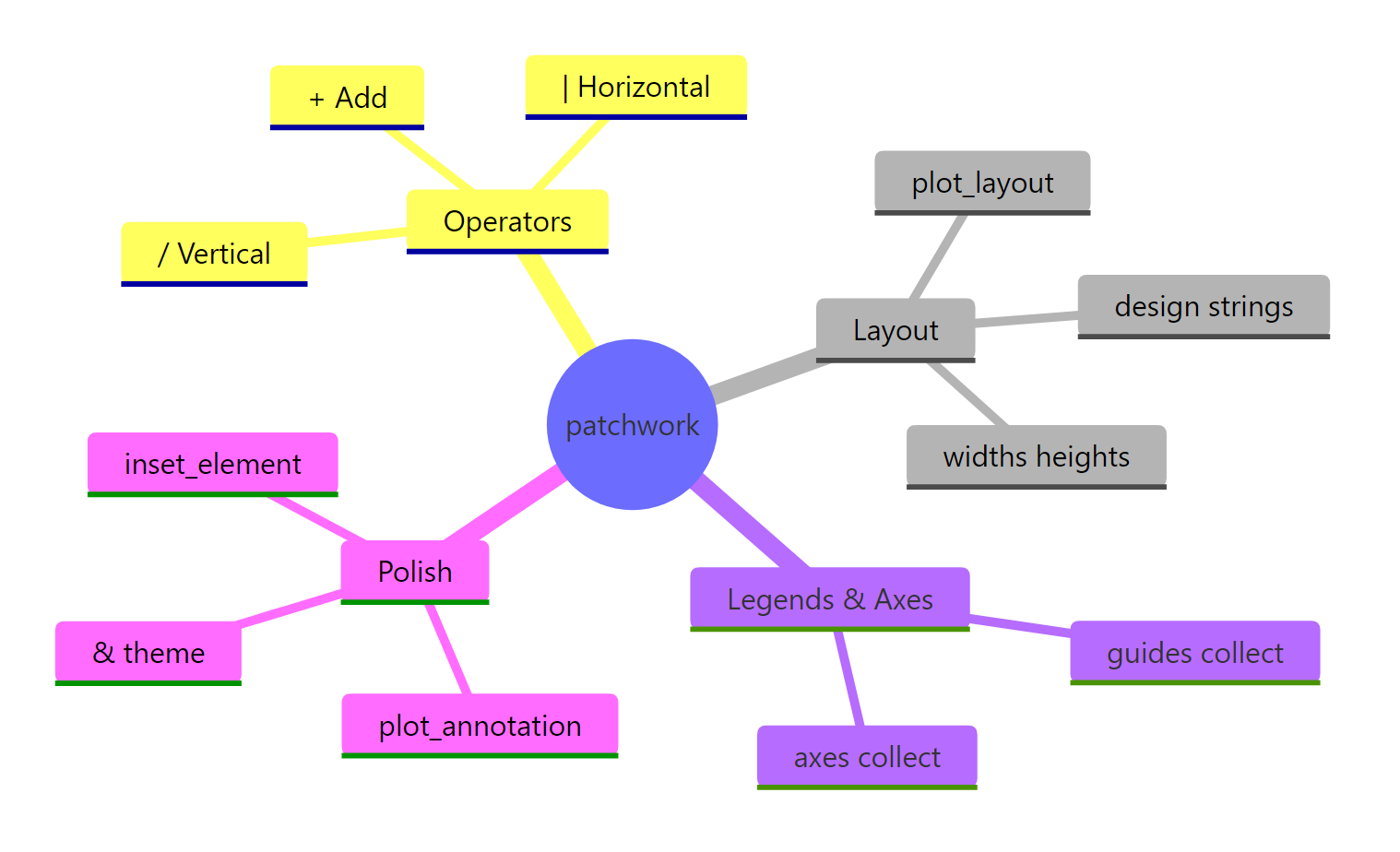
Overview of the patchwork package's main features

Figure 3: Overview of the patchwork package's main features.

References

Pedersen, T.L., patchwork: The Composer of Plots. Official documentation. Link
Pedersen, T.L., Plot Assembly guide (patchwork). Link
Pedersen, T.L., Controlling Layouts (patchwork). Link
Wickham, H., ggplot2: Elegant Graphics for Data Analysis, 3rd ed. Chapter 9: Arranging Plots. Link
CRAN, patchwork package reference manual. Link
Pedersen, T.L., "A small patch of free features" (patchwork 1.2.0 release notes). Link
R Graph Gallery, Combine Multiple Plots with patchwork. Link

Continue Learning

ggplot2 Facets, When you need the same plot repeated across subgroups instead of combining different plots.
ggplot2 Legends, Deep dive into customizing the legends that patchwork collects and aligns.
ggplot2 Labels and Annotations, Master titles, subtitles, and text annotations for individual plots before combining.

patchwork in R: Combine Multiple ggplot2 Plots With Aligned Axes and Shared Legends

How do you combine two ggplot2 plots with patchwork?

How do you control the number of rows and columns?

How do you build complex layouts with nesting and design strings?

How do you share legends and collect axes across plots?

How do you add titles, subtitles, and panel tags?

How do you modify all plots at once with & and *?

How do you add insets and spacers?

Practice Exercises

Exercise 1: Multi-panel iris figure with shared legend

Exercise 2: Diamond dashboard with inset

Exercise 3: Before/after comparison with collected axes

Putting It All Together

Summary

References

Continue Learning

Related Tutorials