Normal, t, F, and Chi-Squared in R: Understand Each Distribution and When It Arises

The Normal, t, F, and Chi-Squared distributions are the four pillars of classical statistics. The Normal models continuous measurements, the Chi-Squared is the distribution of a sum of squared standard normals, the t handles a sample mean when the standard deviation is estimated, and the F compares two variances or tests group effects in ANOVA. In base R you work with all four through the same d/p/q/r function family — no packages required.

How do R's d/p/q/r functions work across every distribution?

Before meeting the four distributions one at a time, it pays to learn the single pattern R uses for every one of them. Base R provides four sibling functions with an identical naming scheme: d for density, p for cumulative probability, q for quantile, and r for random draws. Once you know the pattern on one distribution, it generalises to all of them. Let's try it on the Standard Normal N(0, 1).

RInteractive R

# All four d/p/q/r verbs on the Standard Normal set.seed(1) dnorm(0) # density at x = 0 (peak of the bell) #> [1] 0.3989423 pnorm(1.96) # P(Z <= 1.96) #> [1] 0.9750021 qnorm(0.975) # 97.5th percentile — the 1.96 you know #> [1] 1.959964 rnorm(5) # 5 random draws from N(0, 1) #> [1] -0.6264538 0.1836433 -0.8356286 1.5952808 0.3295078

In one short block you used every verb: dnorm() returned the density height at the peak (about 0.399), pnorm(1.96) gave the famous 97.5% cumulative probability, qnorm(0.975) inverted that to recover 1.96, and rnorm(5) produced five random draws. The payoff is that the exact same four-verb pattern works on the t, Chi-Squared, and F distributions below — only the stem of the function name changes.

The d/p/q/r verb pattern

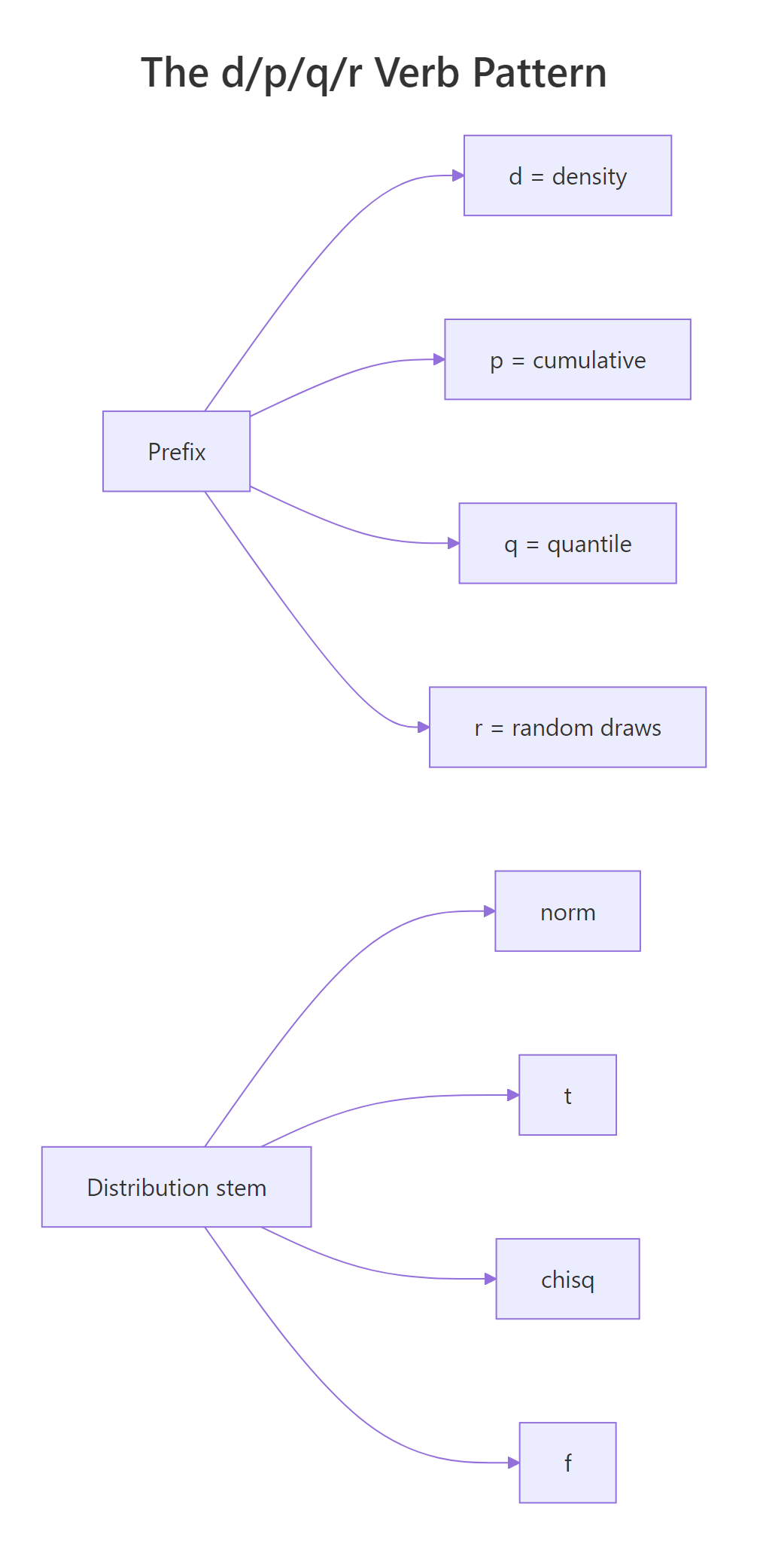
Figure 1: The d/p/q/r verb pattern and the four distribution stems combine to give 16 base-R functions.

The table below pairs each prefix with its job and the kind of return value you should expect.

Prefix	Returns	Input	Output type
`d`	Density (PDF)	A value x	A single density value
`p`	Cumulative probability (CDF)	A value x	A probability in [0, 1]
`q`	Quantile (inverse CDF)	A probability p	The x such that CDF(x) = p
`r`	Random sample	A sample size n	A numeric vector of length n

Tip

Upper-tail probabilities come from lower.tail = FALSE. Instead of writing 1 - pnorm(1.96), call pnorm(1.96, lower.tail = FALSE) directly — it is more accurate for extreme values because subtraction near 1 loses precision.

Try it: Use pnorm() to compute the probability that a Standard Normal random variable is less than −2. Then decide whether that number is a left-tail or upper-tail probability.

RInteractive R

# Try it: left-tail probability at z = -2 ex_p <- NA # your code here ex_p #> Expected: about 0.0228

Click to reveal solution

RInteractive R

ex_p <- pnorm(-2) ex_p #> [1] 0.02275013

Explanation: pnorm() returns the left-tail probability by default — here, P(Z ≤ −2) ≈ 0.023. It is a left-tail probability.

What is the Normal distribution and where does it arise?

The Normal distribution has two parameters: a mean μ that shifts the centre and a standard deviation σ that controls the spread. Its density is bell-shaped and symmetric around μ. Because so many biological and physical measurements cluster around a typical value with smaller and smaller chances of large deviations, the Normal is the default model for continuous data in most fields.

Here is the intuition: the Normal shows up because many independent small influences — genetic effects on height, rounding errors, thermal noise — add up. The Central Limit Theorem tells us that averages of almost anything look Normal once the sample size is large enough.

The density in its full form is:

$$f(x \mid \mu, \sigma) = \frac{1}{\sigma\sqrt{2\pi}} \exp\!\left( -\frac{(x-\mu)^2}{2\sigma^2} \right)$$

Where:

$\mu$ = the mean (centre of the bell)
$\sigma$ = the standard deviation (width of the bell)
$\exp$ = the exponential function

Let's plot the density of a Standard Normal and locate its two-tailed 95% critical value.

RInteractive R

# Plot the Standard Normal density and mark +/- 1.96 curve(dnorm(x), from = -4, to = 4, ylab = "density", main = "Standard Normal N(0, 1)") abline(v = c(-1.96, 1.96), col = "steelblue", lty = 2) # Two-tailed probability outside [-1.96, 1.96] 2 * pnorm(-1.96) #> [1] 0.04999579 # 97.5th percentile — the classic z* for 95% CIs qnorm(0.975) #> [1] 1.959964

The two dashed lines at ±1.96 enclose roughly 95% of the Normal's mass, leaving about 2.5% in each tail. That is why the 95% confidence interval for a mean with a known σ uses z* = 1.96 — it is just qnorm(0.975). A value beyond ±1.96 in standard-normal units is conventionally called "statistically unusual."

Key Insight

Sample means of almost anything follow an approximate Normal. The Central Limit Theorem makes the Normal the limiting distribution for averages, regardless of the original data's shape. That is why the Normal appears far more often in data analysis than its underlying assumptions would suggest.

Try it: IQ scores are modelled as Normal with mean 100 and standard deviation 15. What is the probability that a randomly chosen person has an IQ above 130?

RInteractive R

# Try it: P(IQ > 130) for Normal(100, 15) ex_iq_mu <- 100 ex_iq_sd <- 15 ex_p_iq <- NA # your code here ex_p_iq #> Expected: about 0.0228

Click to reveal solution

RInteractive R

ex_iq_mu <- 100 ex_iq_sd <- 15 ex_p_iq <- pnorm(130, mean = ex_iq_mu, sd = ex_iq_sd, lower.tail = FALSE) ex_p_iq #> [1] 0.02275013

Explanation: An IQ of 130 is exactly 2 standard deviations above the mean, so the upper-tail probability is the same as P(Z > 2) ≈ 0.023.

What is the Chi-Squared distribution and where does it arise?

The Chi-Squared distribution with k degrees of freedom is the distribution of a sum of k squared independent standard normals. It has a single parameter — the degrees of freedom — and takes only non-negative values because you are summing squares. The shape is right-skewed for small k and becomes more symmetric as k grows.

If $Z_1, Z_2, \ldots, Z_k$ are independent N(0, 1), then:

$$\sum_{i=1}^{k} Z_i^{2} \;\sim\; \chi^2_{k}$$

Where:

$Z_i$ = the i-th standard normal random variable
$k$ = the number of terms being summed, equal to the degrees of freedom

Let's verify the genesis definition with a simulation. We'll square 5 standard normals 10,000 times, sum each batch, and check that the resulting histogram matches dchisq(x, df = 5).

RInteractive R

# Build chi-squared(5) by summing 5 squared standard normals set.seed(42) k_df <- 5 chi_samples <- replicate(10000, sum(rnorm(k_df)^2)) hist(chi_samples, breaks = 60, probability = TRUE, col = "lightgray", border = "white", main = "Simulated sum of 5 squared Z's vs. dchisq(x, df = 5)", xlab = "x") curve(dchisq(x, df = 5), from = 0, to = 25, add = TRUE, col = "firebrick", lwd = 2)

The red curve from dchisq() tracks the histogram almost perfectly — confirming that the Chi-Squared really is a sum-of-squared-normals. This genesis is also why Chi-Squared appears whenever you work with sums of squared deviations, like $(n-1)s^2/\sigma^2$ or the Pearson goodness-of-fit statistic.

Now let's compute a critical value and a p-value.

RInteractive R

# Chi-squared critical value at alpha = 0.05 for df = 5 chi_crit <- qchisq(0.95, df = 5) chi_crit #> [1] 11.0705 # P(chi-squared_5 > 7.3) — upper-tail p-value pchisq(7.3, df = 5, lower.tail = FALSE) #> [1] 0.1993315

A test statistic of 7.3 sits inside the non-rejection region because 7.3 < 11.07, and the upper-tail p-value of about 0.20 says the same thing. In a goodness-of-fit test this would mean the observed data is consistent with the hypothesised model.

Note

Chi-squared mean equals df; variance equals twice df. A Chi-Squared with 10 degrees of freedom has mean 10 and variance 20. That is a handy sanity check for any simulation output.

Try it: Find the 95th-percentile critical value of a Chi-Squared with 10 degrees of freedom.

RInteractive R

# Try it: qchisq at 0.95 with df = 10 ex_chi_crit <- NA # your code here ex_chi_crit #> Expected: about 18.31

Click to reveal solution

RInteractive R

ex_chi_crit <- qchisq(0.95, df = 10) ex_chi_crit #> [1] 18.30704

Explanation: For a chi-squared test with 10 degrees of freedom, a test statistic above ~18.31 lands in the rejection region at α = 0.05.

What is the t distribution and where does it arise?

The t distribution looks almost like a Normal but has heavier tails — meaning large values are more likely. It arises when you scale a standard normal by an estimated standard deviation instead of a known one. Formally, if Z ~ N(0, 1) and W ~ χ²_k are independent:

$$t_k = \frac{Z}{\sqrt{W / k}}$$

Where:

$Z$ = a standard normal (the numerator carries the mean signal)
$W$ = a chi-squared with k degrees of freedom (the denominator estimates the variance)
$k$ = degrees of freedom of the t, inherited from W

As k grows, W / k stabilises near 1 and the t converges to the Standard Normal. That convergence is quick: at df = 30 the t and Normal are almost indistinguishable.

RInteractive R

# Overlay t densities at several df against the Standard Normal curve(dnorm(x), from = -4, to = 4, lwd = 2, col = "black", ylab = "density", main = "t(df) approaches Normal as df grows") curve(dt(x, df = 30), from = -4, to = 4, add = TRUE, lwd = 2, col = "steelblue") curve(dt(x, df = 5), from = -4, to = 4, add = TRUE, lwd = 2, col = "darkorange") curve(dt(x, df = 2), from = -4, to = 4, add = TRUE, lwd = 2, col = "firebrick") legend("topright", legend = c("Normal", "t(df=30)", "t(df=5)", "t(df=2)"), col = c("black", "steelblue", "darkorange", "firebrick"), lwd = 2, bty = "n")

The t(df = 2) curve has visibly fatter tails than the Normal — so the same probability mass spreads further out, inflating critical values.

Now the small-sample 95% CI critical value:

RInteractive R

# 95% critical value for a 10-sample t-test (df = n - 1 = 9) qt(0.975, df = 9) #> [1] 2.262157 # Compare to the Normal's 1.96 qnorm(0.975) #> [1] 1.959964

For n = 10, the correct two-sided 95% cutoff is about 2.26, noticeably larger than 1.96. That extra width is the price you pay for not knowing σ — the t distribution protects you against under-estimating uncertainty at small sample sizes.

Warning

Don't reuse 1.96 when your sample size is small. With n = 5 the correct critical value is qt(0.975, df = 4) ≈ 2.78, and a confidence interval built on 1.96 would be roughly 30% too narrow. Call qt() for confidence intervals whenever σ is estimated.

Try it: Compute the 95% two-sided t critical value for a very small sample with 4 degrees of freedom, and compare it to 1.96.

RInteractive R

# Try it: qt at 0.975 with df = 4 ex_t_crit <- NA # your code here ex_t_crit #> Expected: about 2.776

Click to reveal solution

RInteractive R

ex_t_crit <- qt(0.975, df = 4) ex_t_crit #> [1] 2.776445

Explanation: With only 5 observations the 95% t critical value is about 2.78 — much wider than the 1.96 you would use if σ were known.

What is the F distribution and where does it arise?

The F distribution is the ratio of two independent scaled Chi-Squared random variables. If W1 ~ χ²(d1) and W2 ~ χ²(d2) are independent, then:

$$F_{d_1, d_2} = \frac{W_1 / d_1}{W_2 / d_2}$$

Where:

$d_1$ = numerator degrees of freedom
$d_2$ = denominator degrees of freedom
$W_1, W_2$ = independent chi-squared random variables

The F takes only non-negative values and is right-skewed. It has two degree-of-freedom parameters, which is why ANOVA tables always report something like F(2, 27).

Let's confirm the genesis by simulation. We'll construct F samples from two chi-squared samples and overlay the theoretical density.

RInteractive R

# Build F(3, 27) as a ratio of scaled chi-squareds set.seed(123) d1 <- 3 d2 <- 27 chi_num <- rchisq(10000, df = d1) chi_den <- rchisq(10000, df = d2) f_samples <- (chi_num / d1) / (chi_den / d2) hist(f_samples, breaks = 80, probability = TRUE, col = "lightgray", border = "white", xlim = c(0, 6), main = "Simulated chi-sq ratio vs. df(x, 3, 27)", xlab = "x") curve(df(x, df1 = d1, df2 = d2), from = 0, to = 6, add = TRUE, col = "firebrick", lwd = 2)

The theoretical curve from df() sits right on top of the simulated histogram — so the F really is a ratio of scaled chi-squareds. That ratio structure is what makes the F the natural yardstick for questions that compare variances.

Now an ANOVA critical value. Suppose you have 3 groups (so d1 = 3 - 1 = 2) and 30 total observations (so d2 = 30 - 3 = 27).

RInteractive R

# ANOVA critical value at alpha = 0.05 for 3 groups, n = 30 qf(0.95, df1 = 2, df2 = 27) #> [1] 3.354131 # P(F > 4) for the same df — a stylised observed F pf(4, df1 = 2, df2 = 27, lower.tail = FALSE) #> [1] 0.03024462

A computed F of 4 exceeds the critical value of 3.35, and the p-value of about 0.030 is below 0.05, so the null of equal group means would be rejected.

Tip

Don't shadow R's F density function with a variable named df. The letters df are one of R's most common user-variable names, but they also name the F density function. If you ever see a confusing error, call stats::df() explicitly or rename your data frame.

Try it: Compute the upper-tail p-value of F = 4 with df1 = 2, df2 = 27 using pf().

RInteractive R

# Try it: upper-tail p-value for F = 4 ex_f_p <- NA # your code here ex_f_p #> Expected: about 0.030

Click to reveal solution

RInteractive R

ex_f_p <- pf(4, df1 = 2, df2 = 27, lower.tail = FALSE) ex_f_p #> [1] 0.03024462

Explanation: With lower.tail = FALSE, pf() returns the probability that F exceeds 4 — exactly the p-value an ANOVA would report for this test statistic.

How are Normal, t, F, and Chi-Squared distributions connected?

Once you see the chain in Figure 2, the four distributions stop feeling like a loose set of names and start feeling like one system built on the Standard Normal.

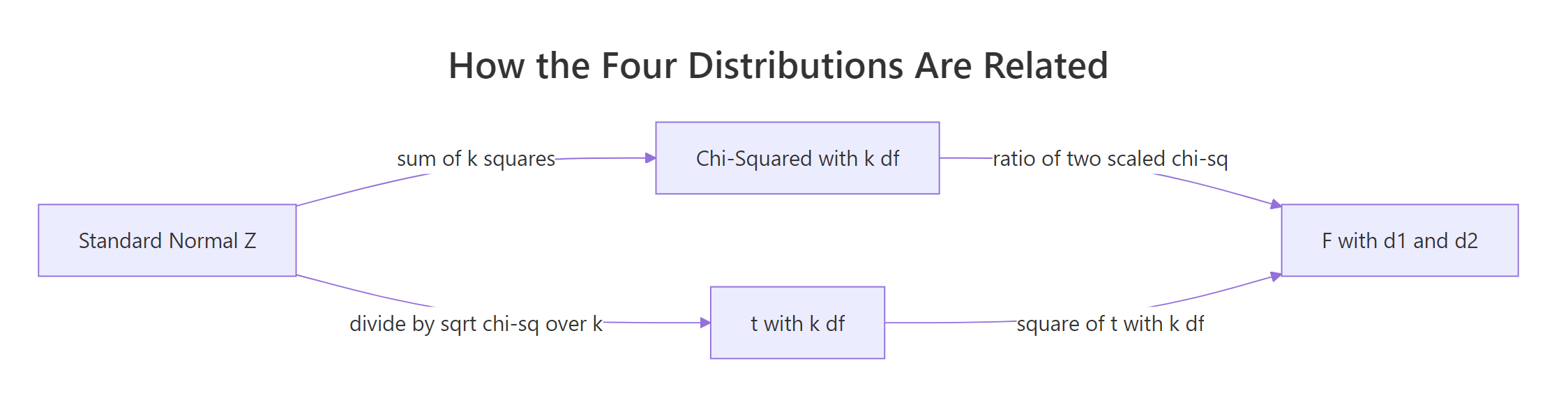
Genesis chain of the four distributions

Figure 2: Every classical distribution descends from the Standard Normal.

Read the chain like this: start with N(0, 1). Square-and-sum k of those to get χ²_k. Then divide a new Z by √(χ²_k / k) to get t_k.

Take the ratio of two scaled chi-squareds to get F(d1, d2). And if you square a t_k, you land back on F(1, k) — because the numerator Z² is itself χ²_1.

Relationship	In symbols
Chi-Squared from Normal	$\sum_{i=1}^k Z_i^2 \sim \chi^2_k$
t from Normal and Chi-Squared	$t_k = Z / \sqrt{W / k}$, where $W \sim \chi^2_k$
F from two Chi-Squareds	$F_{d_1, d_2} = (W_1/d_1) / (W_2/d_2)$
t squared equals F(1, k)	$t_k^2 \sim F_{1, k}$
t at infinity	$t_\infty = Z$

Let's check the t² = F(1, k) identity empirically.

RInteractive R

# Square 10,000 draws from t(10) and compare to F(1, 10) set.seed(7) t_draws <- rt(10000, df = 10) hist(t_draws^2, breaks = 120, probability = TRUE, xlim = c(0, 10), col = "lightgray", border = "white", main = "t(10) squared vs. F(1, 10) density", xlab = "x") curve(df(x, df1 = 1, df2 = 10), from = 0, to = 10, add = TRUE, col = "firebrick", lwd = 2)

The simulated histogram of t_draws^2 sits right under the theoretical F(1, 10) curve — an exact algebraic identity, now visible.

Key Insight

Four distributions cover most classical inference because inference is about means and variances. The Normal carries a signal, the Chi-Squared measures a sum of squared deviations, the t combines them when σ is estimated, and the F compares two of them. Almost every classical test reduces to one of these four.

Try it: Use pnorm() two different ways to compute P(Z < −2): once directly with pnorm(-2), and once via 1 - pnorm(2). Confirm they agree.

RInteractive R

# Try it: two routes to the same tail probability ex_p_direct <- NA # pnorm(-2) ex_p_compl <- NA # 1 - pnorm(2) c(ex_p_direct, ex_p_compl) #> Expected: about 0.0228 twice

Click to reveal solution

RInteractive R

ex_p_direct <- pnorm(-2) ex_p_compl <- 1 - pnorm(2) c(ex_p_direct, ex_p_compl) #> [1] 0.02275013 0.02275013

Explanation: By symmetry of the Normal, P(Z < −2) equals P(Z > 2). The direct call is usually preferred because it avoids precision loss when subtracting a probability close to 1.

Practice Exercises

Exercise 1: Build a 95% t confidence interval and compare to a Normal-based one

For a sample with n = 25, mean 52, and sample standard deviation 8, build a 95% confidence interval for the mean using the t distribution. Then build the same interval using the Normal's 1.96 cutoff and report how much wider the t-based interval is.

RInteractive R

# Your code below — produce my_tci and my_zci my_mean <- 52 my_sd <- 8 my_n <- 25 # my_tci <- ... # my_zci <- ...

Click to reveal solution

RInteractive R

my_mean <- 52 my_sd <- 8 my_n <- 25 my_se <- my_sd / sqrt(my_n) my_tci <- my_mean + qt(c(0.025, 0.975), df = my_n - 1) * my_se my_zci <- my_mean + qnorm(c(0.025, 0.975)) * my_se my_tci #> [1] 48.69740 55.30260 my_zci #> [1] 48.86402 55.13598 # Width comparison diff(my_tci) / diff(my_zci) #> [1] 1.053135

Explanation: The t-based CI is about 5% wider because qt(0.975, df = 24) ≈ 2.064 exceeds 1.96. Using the Normal with an estimated σ would understate your uncertainty.

Exercise 2: Verify the genesis of the Chi-Squared by two simulation routes

Generate 5,000 Chi-Squared(8) samples two ways: (a) directly with rchisq(), and (b) by summing 8 squared standard normals per draw. Plot both histograms on the same axes and confirm they align.

RInteractive R

# Your code below — produce my_rchi and my_sumsq set.seed(2026) my_rchi <- NA # direct rchisq route my_sumsq <- NA # sum-of-squared-Z route

Click to reveal solution

RInteractive R

set.seed(2026) my_rchi <- rchisq(5000, df = 8) my_sumsq <- replicate(5000, sum(rnorm(8)^2)) hist(my_rchi, breaks = 60, probability = TRUE, col = rgb(0.2, 0.4, 0.8, 0.4), border = NA, main = "rchisq vs. sum of squared Z's", xlab = "x") hist(my_sumsq, breaks = 60, probability = TRUE, col = rgb(0.8, 0.2, 0.2, 0.4), border = NA, add = TRUE) # Compare sample means (both should be ~8 = df) c(mean(my_rchi), mean(my_sumsq)) #> [1] 8.011 7.986

Explanation: The two histograms overlap closely and both sample means hover near 8, confirming that a Chi-Squared with k degrees of freedom is literally a sum of k squared standard normals.

Exercise 3: Decide on an ANOVA from an observed F

An ANOVA on 4 groups with 40 observations returns an observed F of 3.2. Compute the 5% critical value and the p-value, and decide whether to reject the null of equal group means.

RInteractive R

# Your code below — produce my_fcrit and my_fp my_groups <- 4 my_n_obs <- 40 my_fstat <- 3.2 # my_fcrit <- ... # my_fp <- ...

Click to reveal solution

RInteractive R

my_groups <- 4 my_n_obs <- 40 my_fstat <- 3.2 my_d1 <- my_groups - 1 # numerator df my_d2 <- my_n_obs - my_groups # denominator df my_fcrit <- qf(0.95, df1 = my_d1, df2 = my_d2) my_fp <- pf(my_fstat, df1 = my_d1, df2 = my_d2, lower.tail = FALSE) c(df1 = my_d1, df2 = my_d2, fcrit = my_fcrit, fp = my_fp) #> df1 df2 fcrit fp #> 3.0000000 36.0000000 2.8662659 0.0347240

Explanation: Since 3.2 > 2.87 and p ≈ 0.035 < 0.05, you reject the null at α = 0.05 — the group means differ.

Putting It All Together

Let's run one compact analysis that touches all four distributions. The sleep dataset has 10 patients measured on two drugs, and we'll apply Normal, t, F, and Chi-Squared tools to it.

RInteractive R

# All four distributions on one tiny dataset data(sleep) # Paired t-test on the difference — uses the t distribution t_res <- t.test(extra ~ group, data = sleep, paired = TRUE) # Verify the CI critical value by hand using qt() qt_crit <- qt(0.975, df = t_res$parameter) # F-test for equal variances between the two groups var_res <- var.test(extra ~ group, data = sleep) # Normal z-score reference for the observed t statistic (large-sample approximation) z_tail <- pnorm(abs(t_res$statistic), lower.tail = FALSE) * 2 # Chi-squared goodness-of-fit on sign(difference) — are +/- 50/50? diff_extra <- with(sleep, extra[group == 2] - extra[group == 1]) chi_res <- chisq.test(c(sum(diff_extra > 0), sum(diff_extra < 0)), p = c(0.5, 0.5)) list(t_statistic = unname(t_res$statistic), qt_crit = qt_crit, var_F = unname(var_res$statistic), z_tail_2sided = unname(z_tail), chi_sq_pvalue = chi_res$p.value) #> $t_statistic #> [1] -4.062128 #> $qt_crit #> [1] 2.262157 #> $var_F #> [1] 0.7977017 #> $z_tail_2sided #> [1] 4.86e-05 #> $chi_sq_pvalue #> [1] 0.003892417

The paired t-test's statistic of −4.06 exceeds the t(9) critical value of ±2.26, so drug 2 delivers more extra sleep than drug 1. var.test() returns an F statistic of 0.80 — well within the central bulk of F(9, 9), so the variances look similar. A Chi-Squared goodness-of-fit on the signs of the differences also rejects a 50/50 split, a fully non-parametric confirmation of the same conclusion. Four distributions, one dataset, one coherent story.

Summary

When to use which distribution

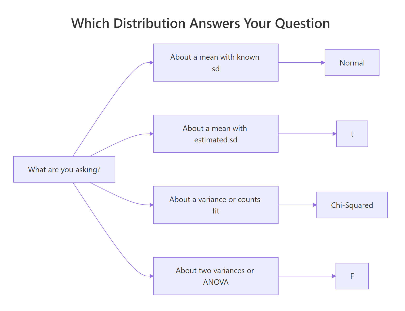
Figure 3: A quick decision guide — which distribution matches which question.

Distribution	Parameters	Typical question	Key R functions
Normal	mean μ, sd σ	Where does a continuous measurement sit relative to its mean?	`dnorm`, `pnorm`, `qnorm`, `rnorm`
Chi-Squared	df k	Is a sum of squared deviations unusually large?	`dchisq`, `pchisq`, `qchisq`, `rchisq`
t	df k	Where does a sample mean sit when σ is estimated?	`dt`, `pt`, `qt`, `rt`
F	df1, df2	Do two variances, or group means, differ?	`df`, `pf`, `qf`, `rf`

Key takeaways:

The d/p/q/r verb pattern works on every base-R distribution — learn it once, reuse it always.
The Normal is the foundation. Chi-Squared sums its squares, t divides by a square-root of chi-squared-over-df, F ratios two chi-squareds.
Use qt() — not 1.96 — whenever σ is estimated from the sample, especially at small n.
An F statistic above the qf(1 - alpha, d1, d2) critical value says the numerator variance is unusually large compared to the denominator.

References

R Core Team — An Introduction to R, §8 "Probability distributions." Link
Base R ?Distributions manual — overview of the d/p/q/r convention. Link
Student (W.S. Gosset) — The Probable Error of a Mean, Biometrika 6(1), 1908. Link
R.A. Fisher — Statistical Methods for Research Workers, introducing the F distribution. Link
Casella, G. & Berger, R.L. — Statistical Inference (2nd ed., Duxbury, 2001), Chapter 5 — chi-squared, t, F genesis derivations.
Venables, W.N. & Ripley, B.D. — Modern Applied Statistics with S (4th ed., Springer, 2002).
Wikipedia — Chi-squared distribution. Link
Wikipedia — F-distribution. Link

Continue Learning

Random Variables in R — foundation concepts for PMFs, PDFs, and expectations that power every distribution on this page.
Binomial vs Poisson in R — the discrete counterparts when you are counting events instead of measuring magnitudes.
Statistical Tests in R — put the Normal, t, F, and Chi-Squared to work in real hypothesis tests.

Normal, t, F, and Chi-Squared in R: Understand Each Distribution and When It Arises

How do R's d/p/q/r functions work across every distribution?

What is the Normal distribution and where does it arise?

What is the Chi-Squared distribution and where does it arise?

What is the t distribution and where does it arise?

What is the F distribution and where does it arise?

How are Normal, t, F, and Chi-Squared distributions connected?

Practice Exercises

Exercise 1: Build a 95% t confidence interval and compare to a Normal-based one

Exercise 2: Verify the genesis of the Chi-Squared by two simulation routes

Exercise 3: Decide on an ANOVA from an observed F

Putting It All Together

Summary

References

Continue Learning

Related Tutorials